Fluid Flow in Pipes — Reynolds Number & Darcy-Weisbach Pressure Drop

Name: Fluid Flow in Pipes — Reynolds Number and Darcy-Weisbach Calculator
Author: MechSimulator

Pipe Flow: The Foundation of Fluid Engineering

Every water distribution network, oil pipeline, HVAC duct, hydraulic circuit, and chemical plant relies on the same fundamental question: given a fluid, a pipe, and a flow rate, what is the pressure drop? The answer determines pump sizing, pipe diameter selection, and energy cost over the life of the system. Get it wrong and pumps cavitate, flows stagnate, or pipes burst.

Two quantities govern the answer — the Reynolds number (which tells you whether the flow is smooth and orderly or chaotic and turbulent) and the Darcy friction factor (which quantifies how much the pipe wall resists the flow). The MechSimulator Fluid Flow Calculator computes both in real time, displays the animated velocity profile and hydraulic grade line, and reports major and minor head losses separately for water, oil, air, and glycerin across four common pipe materials.

The Reynolds Number — Laminar vs Turbulent Flow

The Reynolds number is the dimensionless ratio of inertial to viscous forces in the flow:

\text{Re} = \frac{\rho V D}{\mu}

where ρ is fluid density (kg/m³), V is mean velocity (m/s), D is pipe internal diameter (m), and μ is dynamic viscosity (Pa·s). Three regimes:

Laminar (Re < 2300) — fluid moves in parallel layers; the velocity profile is a perfect parabola (maximum at centreline, zero at wall). Very predictable.
Transitional (2300 < Re < 4000) — unstable, intermittently laminar and turbulent. Avoid this regime in design.
Turbulent (Re > 4000) — chaotic eddies mix the fluid; flatter velocity profile, much higher friction. Most industrial pipe flows are turbulent.

The simulator displays the animated velocity profile in the pipe cross-section — parabolic for laminar, blunted for turbulent — so the difference is immediately visible.

The Darcy-Weisbach Equation

Once the friction factor is known, the major head loss along a pipe of length L is:

h_f = f \cdot \frac{L}{D} \cdot \frac{V^2}{2g}

The corresponding pressure drop is:

\Delta P = \rho g h_f

Friction Factor for Laminar Flow

For laminar flow, friction factor is derived analytically and is exact:

f = \frac{64}{\text{Re}}

Crucially, pipe roughness has no effect on laminar friction — the viscous sublayer completely masks wall irregularities.

Friction Factor for Turbulent Flow: Colebrook Equation

For turbulent flow, the Colebrook equation (used to build the Moody diagram) relates f to both Re and relative roughness ε/D:

\frac{1}{\sqrt{f}} = -2\log\!\left(\frac{\varepsilon}{3.7D} + \frac{2.51}{\text{Re}\sqrt{f}}\right)

This implicit equation is solved iteratively. The explicit Swamee-Jain approximation (accurate to ±1%) is often used in practice:

f \approx \frac{0.25}{\left[\log\!\left(\dfrac{\varepsilon}{3.7D} + \dfrac{5.74}{\text{Re}^{0.9}}\right)\right]^2}

Minor Losses

Head loss at each bend, valve, or fitting:

h_m = K \cdot \frac{V^2}{2g}

where K is a loss coefficient (K ≈ 0.9 for a standard 90° bend, K ≈ 0.5 for a sharp entry). Total system head loss = h_f + Σh_m.

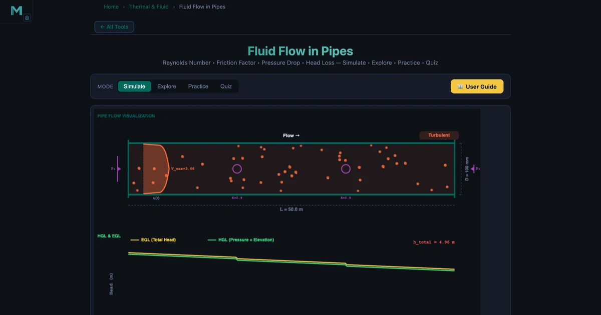
Worked Example: Turbulent Water Flow

Load the Turbulent Flow preset: water (ρ = 998 kg/m³, μ = 1.002 × 10⁻³ Pa·s) in commercial steel pipe (ε = 0.045 mm), D = 100 mm, V = 3 m/s, L = 50 m, 2 bends.

Reynolds number: Re = 998 × 3 × 0.1 / 0.001002 = 298,802 → Turbulent.

Relative roughness: ε/D = 0.045/100 = 0.00045. From the Colebrook equation (solved iteratively): f = 0.0180.

Major head loss: h_f = 0.0180 × (50/0.1) × (9/19.62) = 4.14 m. Minor losses (2 × K = 0.9): h_m = 2 × 0.9 × 9/19.62 = 0.826 m. Total head loss: 4.97 m.

Pressure drop: ΔP = 998 × 9.81 × 4.97 = 48,590 Pa ≈ 48.6 kPa. Flow rate: Q = 3 × π × 0.01/4 = 23.6 L/s.

These match the simulator readouts exactly: Re = 298,802, f = 0.0180, ΔP = 48.59 kPa, h_f = 4.138 m, h_m = 0.826 m, Q = 23.56 L/s ✓.

Laminar Oil Flow: A Very Different Regime

Switch to the Laminar Flow preset: oil (ρ = 880 kg/m³, μ = 0.08 Pa·s) in a smooth pipe, D = 25 mm, V = 0.2 m/s, L = 5 m.

Reynolds number: Re = 880 × 0.2 × 0.025 / 0.08 = 55 → strongly laminar. Friction factor: f = 64/55 = 1.164 — notice how much larger f is than the turbulent value of 0.018. This does not mean more friction; it means laminar friction grows with 1/Re.

Head loss: h_f = 1.164 × (5/0.025) × (0.04/19.62) = 0.474 m. Pressure drop: ΔP = 880 × 9.81 × 0.474 = 4,090 Pa ≈ 4.1 kPa.

Despite a friction factor 65× larger than the turbulent case, the pressure drop is only 4.1 kPa versus 48.6 kPa for turbulent water. Why? The velocity is 15× lower (0.2 vs 3 m/s), the pipe diameter is 4× smaller (25 vs 100 mm), and head loss scales as V² — the combined effect of lower velocity and shorter, narrower pipe completely dominates over the higher friction factor.

Pipe Roughness and the Moody Diagram

Roughness matters only in turbulent flow, and its effect increases with Re until the "fully rough" regime is reached at very high Reynolds numbers. The four pipe materials in the simulator span nearly three orders of magnitude in roughness:

Smooth / drawn pipe — ε ≈ 0. Only hydrodynamically smooth at low to moderate Re.
PVC — ε = 0.0015 mm. Very low roughness, effectively smooth for most HVAC and water service flows.
Commercial steel — ε = 0.045 mm. Standard for industrial piping, water mains, gas distribution.
Cast iron — ε = 0.26 mm. Old water mains, 170× rougher than PVC. Tuberculation with age can increase effective roughness to 1–3 mm.

Try keeping the Turbulent preset conditions and switching only the pipe material. Observe how friction factor and pressure drop change. Then switch to laminar conditions — notice that the pipe material selector has no effect on f = 64/Re.

Using the Fluid Flow Simulator

Open the Fluid Flow in Pipes Calculator and work through these:

Reynolds number sensitivity — Fix all parameters at the turbulent preset. Halve the velocity to 1.5 m/s. Re halves (≈ 149,000). Does the flow remain turbulent? How does the friction factor change?
Diameter effect on head loss — The Darcy-Weisbach equation shows h_f ∝ V²/D. But at constant flow rate Q, V ∝ 1/D², so h_f ∝ 1/D⁵. Double the diameter from 50 to 100 mm at constant Q and watch head loss drop by a factor of 32.
Minor losses dominate short systems — Use the High Loss System preset (8 bends, L = 100 m, V = 5 m/s, cast iron). Compare h_f vs h_m. At high velocity and many fittings, minor losses become significant.
Air duct design — Load the Air Duct preset (air, smooth, D = 300 mm, V = 8 m/s, L = 20 m). Note the low density of air means very low pressure drop in Pa even at high velocity — but HVAC fan power P = Q × ΔP adds up quickly over long duct runs.

Key Takeaways

Re = ρVD/μ determines the flow regime. Below 2300: laminar, f = 64/Re, roughness irrelevant. Above 4000: turbulent, use Colebrook or Moody diagram, roughness matters.
Head loss scales with V². Doubling flow velocity quadruples friction losses — pipe diameter is the most powerful design variable for reducing energy consumption.
h_f ∝ 1/D⁵ at constant flow rate. A modest increase in pipe diameter delivers enormous reductions in head loss — justifying the extra material cost in long pipelines.
Roughness only matters in turbulent flow. Laminar friction (f = 64/Re) is independent of pipe material and entirely controlled by viscosity and velocity.
Don't neglect minor losses. In short, high-velocity systems with many fittings, minor losses (bends, valves, entries) can exceed major friction losses.

Explore Related Simulators

Pipe flow theory connects directly to real system design. The Bernoulli's Principle — Fluid Dynamics guide covers the energy balance that underpins the hydraulic grade line visible in the simulator — understanding Bernoulli alongside Darcy-Weisbach gives a complete picture of pipe system energy. For hydraulic power systems that use pressurised oil rather than water, the Hydraulic Circuit Simulator shows how flow rate, pressure, and cylinder speed interact in practical circuit layouts.

Frequently Asked Questions

What is the Reynolds number for pipe flow?

Re = ρVD/μ is a dimensionless ratio of inertial to viscous forces. Re < 2300: laminar; Re > 4000: turbulent; 2300–4000: transitional. It is the most important parameter in pipe flow analysis.

What is the Darcy-Weisbach equation?

h_f = f(L/D)(V²/2g), where f is the Darcy friction factor, L is pipe length, D is diameter, V is mean velocity, and g = 9.81 m/s². Pressure drop: ΔP = ρgh_f. Valid for both laminar and turbulent flow with the appropriate f.

How is friction factor calculated for laminar and turbulent flow?

Laminar: f = 64/Re (exact, roughness-independent). Turbulent: use the Colebrook equation (implicit, requires iteration) or Swamee-Jain explicit approximation: f = 0.25/[log(ε/(3.7D) + 5.74/Re⁰·⁹)]².

What is the difference between major and minor head losses?

Major losses: h_f = f(L/D)(V²/2g) — friction along the pipe length. Minor losses: h_m = K(V²/2g) — at fittings, bends, and valves. Minor losses dominate short high-velocity systems; major losses dominate long pipelines.

How does pipe roughness affect pressure drop?

Roughness only affects turbulent flow. Relative roughness ε/D enters the Colebrook equation: smooth (ε ≈ 0), PVC (0.0015 mm), steel (0.045 mm), cast iron (0.26 mm). Cast iron has 170× the roughness of PVC, significantly increasing turbulent friction factor and pressure drop.