Interactive Psychrometric Chart Calculator
Interactive ASHRAE-grade moist-air properties • Click any point • HVAC processes • Coil sizing • Comfort & data-center overlays — Simulate • Explore • Practice • Quiz
i Live Equations — ASHRAE Ch. 1 (Hyland-Wexler)
Industrial Modules
Sizes a cooling coil along the canonical Outdoor → Mix → Coil → Supply path. The room loads and air flow fix the supply state; the coil line from the mixed air through the supply, extended to saturation, gives the apparatus dew point (ADP). RSHF, GSHF and the bypass factor BF = (TS − TADP)/(TM − TADP) are the results. On the chart it draws the textbook diagram: the two mixing lines into M, the coil line M → S extended to the ADP, and the room line S → RA (when the return air is the room state).
Outdoor Air (OA)
Return Air (RA)
Room Loads
Targets
User Guide & Documentation
1 Overview

The Psychrometric Chart Calculator is a professional-grade tool for engineers, technicians, and students who need accurate moist-air properties for HVAC, industrial drying, evaporative cooling, cooling-tower work, data centers, museum/archive conservation and building science. Math is implemented per ASHRAE Handbook of Fundamentals Chapter 1 (Hyland-Wexler saturation pressure with the correct ice/water split at 0 °C).
Four modes — Simulate for free-form chart exploration and property lookup; Explore for theory; Practice for unlimited drill; Quiz for a graded 5-question assessment with star rating.
2 Configuring the System
The chart loads with one state point at 25 °C / 50% RH (sea-level pressure, SI units). Click anywhere on the chart to drop or move the active point; or type any two of Tdb, Twb, Tdp, RH, W, h directly into the Properties panel and the rest update automatically. Use the SI/IP toggle (top-right) at any time — internal math stays in SI; only the display changes.
3 Using the Chart
Chart Explorer. Click to move the active point, or drag any point. With the chart focused (Tab to it), the arrow keys nudge the active point — Shift for ten times the step. Use + Add for up to 5 labelled points (A – E), or + Custom Point to type one from a pair of properties. Pick the active point from the State Point dropdown to edit its properties. Connect (on by default) joins the points in order and lists the change and the load along each line — see Plotting Processes & Loads below. Undo / Redo (Ctrl+Z / Ctrl+Shift+Z) step through point moves, edits, presets, overlays and process changes. Share copies a link that reopens this exact chart.
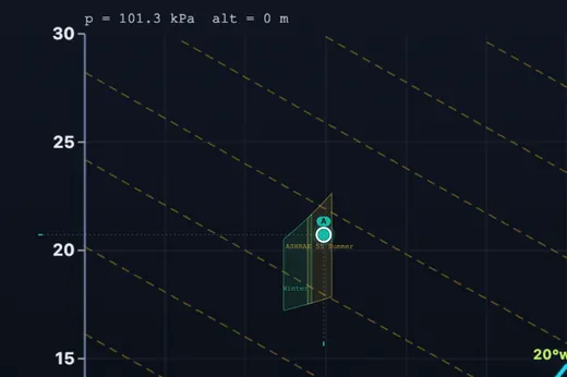
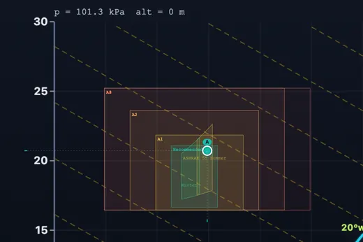
Overlays. Toggle constant wet-bulb, enthalpy and specific-volume lines. The Comfort overlay draws the ASHRAE 55 graphic comfort zone, computed from Fanger’s PMV (−0.5 to +0.5) for 1.1 met, still air (0.1 m/s) and 0.5 clo (summer) or 1.0 clo (winter), up to W = 12 g/kg — which is why its sides slant. The Data Center overlay draws the ASHRAE TC 9.9 (2021) recommended envelope and classes A1 – A4 with both their dew-point and RH limits. With either overlay on, a line under the chart says whether the active point is inside.
HVAC processes. Pick a process tab; it starts from the active point. Sensible heating is a horizontal line. Sensible cooling is horizontal until the dew point, then follows the saturation curve as water condenses. Steam humidification climbs vertically (constant Tdb). Evaporative humidification follows the constant wet-bulb line and cannot go below Twb. Cooling + dehumidification runs to the coil leaving dry-bulb you choose at about 95 % RH. Mixing combines Points A and B with W and h weighted by dry-air mass.
Loads. Set the dry-air mass flow ṁa in the bottom card. The tool reports the sensible, latent and total load for the current process, the condensate rate when water condenses, and the sensible heat ratio. Everything is per kilogram (pound) of dry air — if you start from a volume flow, divide it by the specific volume first.
4 Plotting Processes & Loads (Connect)
Connect (toolbar, on by default) joins the points in the order you made them — A → B → C — with an arrow showing the direction. Add points with + Add or + Custom Point, then move each one to a state: outdoor air, after the coil, after the reheat, and so on.
The table under the chart has one row per line: the change in dry-bulb (ΔT), in moisture (ΔW) and in enthalpy (Δh), the heat added or removed (q) at the dry-air flow set in the Air Mass Flow card, and the sensible heat ratio (SHR = sensible ÷ total). A negative q is heat removed. If moisture falls along a line, the water leaves as condensate and its enthalpy is taken out of the load.
Read the line’s direction: horizontal = sensible heating or cooling; down and to the left = cooling with dehumidification; up and to the left along a wet-bulb line = evaporative cooling. A straight line is the change between two states, not the exact path — air cooled past its dew point really follows the saturation curve (the Cool process draws that path). An SHR above 1 or below 0 means moisture moves against the temperature, for example heating while drying.
5 Industrial Modules
Cooling Coil Sizing. Enter the outdoor air, the return air (with their flows), the room’s sensible and latent loads and the room condition, then press Calculate & Plot. The tool mixes the two streams (M), works out the supply state the loads need (S), extends the coil line to the saturation curve for the apparatus dew point (ADP), and reports RSHF, GSHF, the bypass factor, the coil duty, tonnage and condensate. It draws the textbook diagram on the chart — the two mixing lines, the coil line to the ADP and the room line — and replaces your points while it does (Undo brings them back). If the loads are impossible for the air flow it says why instead of printing a number.
Cooling Tower. From water in/out temperatures, the entering-air wet-bulb, the water flow, the cycles of concentration and the drift, it gives range, approach, effectiveness, heat rejected, evaporation (Perry’s rule, about 0.15% of the flow per °C of range), blowdown and make-up water.
Evap Cooling Designer. Direct, indirect or two-stage evaporative cooling from the outdoor state and the effectiveness ε. The supply approaches the entering wet-bulb; the result shows the sensible cooling, the moisture added and the water evaporated.
24-h Timeline. A simple daily cycle between your minimum and maximum dry-bulb, with RH moving the opposite way, and the hours spent inside the ASHRAE 55 comfort zone or the TC 9.9 recommended envelope — a first look at free-cooling hours. All four modules follow the SI/IP toggle.
6 The Underlying Theory
Four tabs: Basics (what the seven properties mean and why), Formulas (saturation pressure with ice/water split, humidity ratio, enthalpy, wet-bulb iterative solver), Applications (HVAC coil sizing, cooling towers, drying, data centers, museums), Standards (ASHRAE 55, TC 9.9, ISO 7730, altitude correction).
7 Try a Problem
Practice draws a random state and asks you to compute a missing property, in the unit system you have selected. The answer is worked from exactly the numbers the question prints. Tolerance: ±0.3 °C (±0.5 °F) for temperatures, ±1 kJ/kg (±0.5 Btu/lb) for enthalpy and ±2 % for the humidity ratio. Each question is graded once; the score tracks correct / attempted.
Quiz is 5 multiple-choice questions drawn from a bank of 10, with the answer order shuffled every time. It covers property identification, process direction on the chart, comfort-zone reading, data-center envelopes and altitude effects. The result shows your score and a 0 – 5 star rating.
8 Altitude & Pressure
The humidity ratio relation W = 0.621945·pw/(p − pw) is explicitly pressure-dependent. A standard sea-level chart misreads moisture at altitude — the error at Denver (~1610 m, ~83 kPa) is roughly 20%. Use the Altitude slider to set the station elevation; the Pressure slider follows the ASHRAE altitude relation. A warning appears above 750 m. Internal math always uses your selected pressure, so all properties remain correct.
9 SI vs IP Units
Toggle at top-right. SI: °C, kJ/kg dry air, g/kg, kPa, m³/kg, m, kg/s, kW, L/s. IP: °F, Btu/lb dry air, gr/lb (grains per pound), inHg, ft³/lb, ft, lb/h, Btu/h, US gpm. The IP chart is a real IP chart: its wet-bulb, enthalpy and volume lines sit on round °F, Btu/lb and ft³/lb values, and IP enthalpy uses the ASHRAE IP datum (0 °F dry air), so it is not simply the SI number × 0.43. The industrial modules convert their inputs when you switch. Internal state stays in SI, so switching back and forth never drifts. The Live Equations panel and the Step-by-Step Calculation stay in SI — the handbook’s own units — and say so when IP is selected.
10 Engineering Notes & Pitfalls
- Which two fields are used. The solver fixes the state from the last two fields you edited, and says which pair under the panel. (Twb, Tdp) and (h, Twb) are ill-conditioned near saturation, and (Tdp, W) carry the same information — the solver warns about each. Prefer pairs that include Tdb.
- Below 0 °C. Saturation is taken over ice (ASHRAE Eq. 5, switched at the triple point so the curve has no step) and the wet-bulb uses the sublimation form (Eq. 35, 2830 kJ/kg). The “dew point” below freezing is therefore the frost point, and the panel labels it so. Right at 0 °C the ice and water wet-bulb equations can both be satisfied a fraction of a degree apart; the tool reports one of them.
- Wet-bulb vs adiabatic saturation. These match within 0.1 °C in normal HVAC range; the tool returns the thermodynamic (adiabatic saturation) wet-bulb — the canonical ASHRAE definition.
- Supersaturation / fog. A pair that implies RH > 100 % is clipped to saturation and the solver says so; the tool does not model the fog region. A state outside the plotted range (−10 to 50 °C, 0 to 30 g/kg) is kept exactly and shown as an arrow at the chart edge.
- Mass flow. All load equations are per unit mass of dry air. Set ṁa in the dedicated card to get total loads. The latent part is ṁ·ΔW·hfg with hfg = 2501 kJ/kg (1075 Btu/lb); when water condenses, the enthalpy it carries away as liquid is included in the total.
11 Presets, Keyboard & Sharing
Presets load a typical condition into the active point and set the site altitude. The dropdown shows the scenario while the chart is in it, and returns to “Choose scenario” as soon as you move the point or change the altitude. City presets are illustrative afternoons, not design data — for design use the ASHRAE climatic design conditions for your site.
Keyboard. Tab to the chart and use the arrow keys to nudge the active point (Shift for bigger steps). Ctrl+Z / Ctrl+Shift+Z undo and redo. Enter commits a typed property; Escape closes the calculation and custom-point windows.
Sharing and export. Share copies a link that reopens this exact chart — points, lines, process, air flow, overlays and altitude. CSV exports every point’s properties in the units shown; PNG saves the chart as an image. Right-click the chart for the same actions.
12 Validation
Saturation pressure, humidity ratio, wet-bulb, dew point, enthalpy, specific volume and density are checked against PsychroLib (Meyer & Thevenard, 2019 — the open implementation of the ASHRAE Handbook — Fundamentals 2017, Ch. 1) across −10 to 50 °C, 5 – 100 % RH and sea level to 3650 m, and the forward and inverse wet-bulb relations are checked to be the same equation. The comfort zone’s PMV is checked against the ISO 7730 Annex D and ASHRAE 55 validation values; the data-center envelopes against ASHRAE’s 2021 Table 2.1. Every figure the Explore cards, quiz and practice print is re-derived by the same test.
Psychrometric Chart Calculator — Theory, Use Cases & Worked Examples
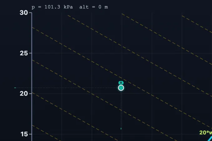
First time I taught psychrometrics, I covered five property lines on the same chart and watched the class fog over. What worked: spend the whole first lesson on just dry-bulb and humidity ratio — locate state points, nothing else. Add wet-bulb the next day. Enthalpy later. By the end of the week the chart is no longer a mess of curves; it's a map. Tools that show all five at once make this harder, not easier, for beginners. Use the layer toggles deliberately.
What a psychrometric chart actually shows
A psychrometric chart is a two-dimensional map of moist air. Pick any two independent properties — usually dry-bulb temperature and either relative humidity or wet-bulb temperature — and every other property (dew point, humidity ratio, enthalpy, specific volume, density) is fixed. For a fixed barometric pressure, two intensive properties determine the state of moist air completely; this is the Gibbs phase rule applied to a single-phase binary mixture of dry air and water vapor.
The chart's seven everyday properties are: dry-bulb temperature (the ordinary thermometer reading), wet-bulb temperature (a wetted-wick thermometer in moving air, simulated thermodynamically by adiabatic saturation), dew point (the temperature at which condensation starts), relative humidity (ratio of water-vapor partial pressure to saturation pressure), humidity ratio W (kilograms of water vapor per kilogram of dry air), enthalpy h (kJ per kilogram of dry air), and specific volume v (cubic metres per kilogram of dry air).
How the math actually works
This tool implements ASHRAE Handbook of Fundamentals Chapter 1 verbatim. Saturation pressure of water vapor is computed by the Hyland-Wexler equations — a seven-constant logarithmic form for ice (−100 to 0 °C) and a six-constant form for liquid water (0 to 200 °C). The split at 0 °C is not cosmetic: the latent heat used in the thermodynamic wet-bulb equation jumps from 2501 kJ/kg (vaporization) to 2830 kJ/kg (sublimation = vaporization + 334 kJ/kg fusion) and the condensate specific heat changes from 4.186 kJ/kg·K (liquid water) to 2.1 kJ/kg·K (ice). Tools that omit this split misread refrigeration and frost-protection problems by several percent.
Humidity ratio is W = 0.621945·pw/(p − pw), where 0.621945 is the molecular-mass ratio Mwater/Mdry air. Older textbooks round to 0.622 or 0.62198 — same physics, lower precision. Specific enthalpy is h = 1.006·t + W·(2501 + 1.86·t) in SI (kJ per kg dry air), or h = 0.240·t + W·(1061 + 0.444·t) in IP (Btu/lb dry air).
Industrial use cases this tool is built for
HVAC cooling-coil sizing is the classic application. Outdoor air mixes with return air at a mass-weighted state; the mixed stream enters the coil and exits along the room sensible-heat ratio (RSHF) line, with the coil’s effective surface temperature (apparatus dew point, ADP) found by extending the process line to the saturation curve. The bypass factor BF = (Tcoil,out − TADP) / (Tcoil,in − TADP) tells you how close the coil approaches ideal. Evaporative cooling follows the constant wet-bulb line — the air’s dry-bulb drops and humidity ratio climbs along a line of constant adiabatic saturation. Cooling tower analysis uses approach (Twater,out − Twb,in) and range to size makeup-water systems. Industrial drying (food, lumber, textile) lives on the chart because the rate of moisture removal depends on the vapor-pressure difference between product and conditioned air.
In data centers, the ASHRAE TC 9.9 envelopes prescribe the air entering the servers: the 2021 recommended envelope is 18–27 °C with a dew point from −9 to 15 °C and at most 70% RH, and Classes A1–A4 widen the allowable range (A1: 15–32 °C, up to 17 °C dew point and 80% RH). Where a dew-point and an RH limit are both given, the tighter one governs, so on the chart the envelopes are curved, never rectangles. Overlay them and check that economizer and humidification strategies keep operation inside year-round. In pharma cleanrooms and museum archives the chart provides the design point for narrow humidity windows (35 – 55% RH typical for paper conservation; ISO 14644 humidity bands for cleanrooms).
Plotting HVAC processes: lines, loads and the apparatus dew point
A single point answers what is this air like? Design work is about a change — outdoor air mixes with return air, passes through a cooling coil and is supplied to the room — and each change is a line between two state points. The direction of the line is the process: horizontal is sensible heating or cooling; down and to the left is cooling with dehumidification (a wet coil); up and to the left along a wet-bulb line is evaporative cooling. The slope is the sensible heat ratio, SHR = qsensible/qtotal.
The load along any line is the enthalpy change times the dry-air mass flow, q = ṁa(h2 − h1), less the enthalpy of any water that condenses; the latent part is ṁa·ΔW·hfg with hfg ≈ 2501 kJ/kg, and the sensible part is the rest. In this tool, Connect joins your points in order and lists ΔT, ΔW, Δh, the load and the SHR for every line, in SI or IP.
Worked example — sizing a cooling coil. Outdoor air at 35 °C, 60% RH (0.34 kg/s) mixes with return air at 24 °C, 50% RH (1.36 kg/s); the room needs 20 kW sensible and 5 kW latent removed. The mixed air M comes out at 26.2 °C and 11.73 g/kg. The room loads fix the supply state S at 12.5 °C and 8.12 g/kg (90% RH). Extending the coil line M → S to the saturation curve gives the apparatus dew point, ADP = 9.3 °C, and the bypass factor BF = (TS − TADP)/(TM − TADP) = 0.19. The coil removes 39.1 kW (11.1 TR) — 23.8 kW sensible and 15.3 kW latent, so its SHR (the GSHF) is 0.61 — and drains about 22 kg of condensate an hour. The room line S → R carries exactly the 25 kW of room load at SHR 0.80, the room sensible heat ratio. The coil does more than the room needs because it also cools and dries the outdoor air. The Cooling Coil Sizing module below draws this whole diagram on the chart.
Is 24 °C at 71% RH comfortable? The ASHRAE 55 comfort zone
ASHRAE Standard 55 does not define comfort as a box of temperature and humidity. Its graphic comfort zone (§5.3.1) is the set of conditions where Fanger’s Predicted Mean Vote (PMV, the ISO 7730 model) lies between −0.5 and +0.5 for a sedentary person (1.1 met) in still air (below 0.2 m/s), wearing 0.5 clo in summer or 1.0 clo in winter — with the humidity ratio no higher than 0.012 kg/kg. There is no lower humidity limit. Because moist air slows evaporation from the skin, the zone’s sides slope toward cooler temperatures as humidity rises.
| Humidity ratio W | Summer, 0.5 clo | Winter, 1.0 clo |
|---|---|---|
| 0 g/kg | 25.0 – 28.3 °C | 21.6 – 26.1 °C |
| 4 g/kg | 24.5 – 27.8 °C | 20.9 – 25.4 °C |
| 8 g/kg | 24.0 – 27.3 °C | 20.2 – 24.7 °C |
| 12 g/kg (limit) | 23.5 – 26.8 °C | 19.5 – 24.0 °C |
So is 24 °C at 71% RH comfortable? Not by ASHRAE 55. Its humidity ratio is 13.3 g/kg, above the 12 g/kg limit — even though the temperature alone is fine (PMV −0.31 in summer clothing, inside ±0.5). It fails on moisture, not warmth: at 24 °C the limit is about 64% RH at sea level. Turn on the Comfort overlay and the tool says whether the active point is inside the zone, and in which season.
Why altitude correction is non-negotiable
Because W depends explicitly on barometric pressure, a sea-level chart cannot be used unmodified at altitude. ASHRAE publishes separate charts for 750, 1500 and 2250 m for exactly this reason. This calculator accepts altitude or barometric pressure as a first-class input, redraws the chart accordingly, and warns the user when sea-level pressure would be misapplied. Engineers in Denver, Mexico City, Johannesburg or any plateau city should always set the correct altitude before sizing equipment.
Who Uses This Simulator?
HVAC design engineers sizing cooling and heating coils, cooling towers, evaporative coolers and dehumidification systems. Mechanical engineering students learning refrigeration & air-conditioning, often working through Stoecker, Cengel or ASHRAE textbook problems. Building energy modellers setting up EnergyPlus / IES VE simulations who need ground-truth state points. Industrial process engineers in food, pharma, paper and lumber drying. Data center operators verifying ASHRAE TC 9.9 envelope compliance. Architects and building scientists evaluating natural ventilation and passive cooling. FE/PE and GATE candidates drilling psychrometric problems.
Explore Related Simulators
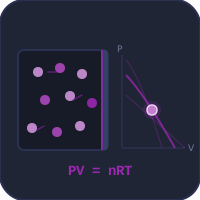
Pair the psychrometric chart with our Refrigeration Cycle Simulator for full vapor-compression COP analysis; the Heat Exchanger Simulator for LMTD/NTU coil sizing; the Ideal Gas Law for the underlying state equation of dry air; and the Specific Heat Capacity Simulator to understand the sensible-heat term in the enthalpy equation.
Updated