
Centrifugal Pump Test Rig Simulator
Plot head-capacity, power & efficiency curves — find the BEP, apply affinity laws, match a system curve and check NPSH on six pump presets


- Start the pump to assess the machine.
📖 User Guide — Centrifugal Pump Test Rig
1 Overview
This virtual centrifugal pump test rig reproduces a complete hydraulics-lab pump bench — a sump, a volute pump with impeller, suction and delivery pipes, vacuum and pressure gauges, a motor with an energy meter, a gate (delivery) valve and a calibrated collecting tank. By throttling the delivery valve you trace the pump's characteristic curves: head-capacity (H–Q), shaft power, and efficiency, and you can locate the best efficiency point (BEP).
The valve is a real hydraulic resistance, not a flow slider. The discharge is solved every frame as the intersection of the pump curve with the system curve, so closing the gate walks the operating point up the H–Q curve, and raising the static lift genuinely reduces the flow. Six pump presets are provided; the impeller diameter, number of stages and rated speed set the machine, and the static suction lift, static delivery lift, site altitude and water temperature set the installation it is bolted into.
Six automated test procedures are bundled (Constant-Speed Characteristic, Combined Characteristic, Variable-Speed / Affinity, Multi-Speed Family, System Curve & Duty Point, and NPSH / Cavitation). Results are shown in seven chart views, a one-click professional PDF report documents each run, and an SI / Imperial toggle (in the control panel, beside Pump Setup) converts head (m ↔ ft), discharge (L/s ↔ gpm), power (kW ↔ hp), volume, temperature and pressure throughout. Four modes — Simulate, Explore, Practice and Quiz — cover hands-on use, theory, numerical practice and self-testing.
2 Getting Started — Run Your First Test

- Pick a pump from the six preset chips (e.g. "3 HP").
- (Optional) Open ⚙ Pump Setup to change the impeller diameter, number of stages and rated speed, and the installation: static suction lift, static delivery lift, site altitude and water temperature. The preview panel shows the resulting shut-off head, BEP, static head, NPSH available and required, and the duty point with the gate wide open — before you commit.
- Click ▶ Prime & Start. The casing fills, the impeller spins and the gauges come alive. Until it is primed the rig shows a NOT PRIMED banner — a centrifugal pump cannot pump air.
- Set the speed N and the delivery-valve opening with the two sliders. Closing the gate adds system resistance, so the head rises and the flow falls; opening it does the reverse. A gate valve moves the flow only gently above about 60 % open and then bites hard, which is why the interesting part of the sweep is the bottom half of the slider.
- Click 🧪 Run Test, choose a procedure, and press Run Test on its card. A progress banner shows the current step; × CANCEL on that banner, or the Esc key, aborts cleanly at any point.
- When it finishes, the results fill the relevant chart and the result cards. Click 📑 Report (PDF) for a printable report, 🧮 Show Calculations for the step-by-step derivation, or CSV / PNG for raw data and images.
The control-panel buttons are: Prime & Start · Run Test · Reset · Pump Setup, followed by the export group (Show Calculations, Report, CSV, PNG). Report and Show Calculations stay disabled until a test has completed. Reset empties the casing as well as clearing the data, so the pump has to be primed again.
3 The Test Rig — Live Instrumentation
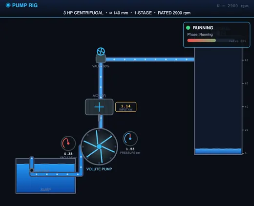
The left canvas is the pump test bed: a sump tank feeds a suction pipe (with a foot valve and strainer) into the eye of the impeller; the volute casing discharges up a delivery pipe through a gate valve to a calibrated collecting tank. A vacuum gauge on the suction side and a pressure gauge on the delivery side give the heads; the motor carries an energy meter for input power. The static suction lift is dimensioned on the drawing, so the Pump Setup value is visible on the rig itself.
The collecting tank is a real measuring device, not decoration. It has a 0.25 m² plan area and 0.60 m of graduated depth, so it holds 150 L, and it fills at the real rate: the panel beneath it shows the volume collected, the elapsed time and the quotient Q = V/t, live. At 3 L/s it takes 50 seconds to fill and then the drain valve opens and the stopwatch restarts — exactly the tank-rise method the Explore tab describes.
A banner across the top-left states any condition worth knowing about: NOT PRIMED, DEAD-HEADING (the pump cannot lift the static head at all, so it delivers nothing), LOW NPSH MARGIN, or ⚠ CAVITATING. When the pump cavitates you also see vapour bubbles forming at the impeller eye and hear the characteristic gravelly noise, and the head visibly breaks down.
The right canvas is the instrument cluster and the characteristic charts. Below them, twenty-two result cards give discharge, total head, water and shaft power, pump and overall efficiency, delivery head, suction lift, specific speed, NPSH available, NPSH required, the NPSH margin, the static head, the rated BEP discharge and the duty as a percentage of it, then the machine-condition readings — vibration with its ISO 10816-7 zone, bearing-housing temperature and seal leakage — and finally the three efficiency terms (volumetric, hydraulic, mechanical) with the wear-ring leakage that drives the first of them. The NPSH-margin, percent-of-BEP, vibration, bearing and seal cards turn amber or red when they leave their safe band.
Under the cards, the Condition assessment panel gives the verdict: the ISO 10816-7 zone, an ALARM or TRIP flag, and the list of actions a maintenance engineer would raise — wear-ring renewal at the “2× rule”, a named bearing defect, coupling alignment, seal leakage against the API 682 allowance, cavitation risk, and where the machine is being run: below the minimum continuous stable flow, outside the API 610 preferred operating region of 70–120 % of rated BEP, or dead-headed against a shut valve. It is the same assessment the exported PDF report and CSV carry.
4 Run Test — Standard Procedures
The 🧪 Run Test button opens the procedure picker. Six procedures are bundled, and every one of them keeps and plots the points it measures:
- Constant-Speed Characteristic Test (IS 9137 / ISO 9906) — at rated speed, starts with the gate shut to fix the shut-off head, then opens it in steps to full flow, recording H, Q and power to build the H–Q, power and efficiency curves and locate the BEP.
- Combined Characteristic Test — the same sweep presented as the classic combined chart with H, P and η against Q on one set of axes, each with its own scale.
- Variable-Speed (Affinity) Test — at a fixed gate position, varies the speed and plots the measured duty points against the affinity prediction, so you can see the gap the static head opens up.
- Multi-Speed Family — runs the constant-speed sweep at several speeds and overlays the H–Q curves to show how the whole characteristic scales.
- System Curve & Duty Point — steps the gate through seven positions and marks each measured duty point on the pump and system curves.
- NPSH / Cavitation Test — increases the discharge, plots NPSH available against NPSH required with the measured points marked, and shades the region where the margin is lost.
A progress banner shows the procedure, the current step and a progress bar. The × CANCEL button on that banner is clickable, and Esc does the same thing. Results route to the right chart automatically.
5 Chart Views
Use the Chart View tabs to switch how results are displayed. The live operating point is marked on every chart where it applies:
- H–Q — the head-capacity curve, solid over the range the rig can actually reach and faint-dashed beyond it, because free delivery is an extrapolation no bench can measure.
- Power — shaft power vs discharge, rising from the shut-off power, which is marked with its own value. It is finite, at about 71 % of the BEP power — not zero.
- Efficiency — efficiency vs discharge, peaking at the best efficiency point, which is read off the curve rather than assumed.
- Combined — H, P and η on one plot with three separate scales: head on the left, power and efficiency on the right.
- System — the pump curve, the static-head line, the system curve at the current gate position and at the gate wide open, and the duty point. This duty point is the live operating point — move the valve slider and watch it slide along the pump curve.
- Affinity — the H–Q family at several speeds, plus the measured duty points against the affinity prediction once the Variable-Speed test has run.
- NPSH — NPSH available vs NPSH required against discharge, with the cavitation region shaded and the current atmospheric and vapour pressures printed.
- Vibration — the spectrum, with the ISO 10816-7 zone bands behind it, every defect standing at its own frequency and the overall RMS marked. This is where you diagnose the machine.
Right-click either canvas for a context menu. On the rig: save the image, copy the current reading, reset. On the chart: copy the operating point, export the readings as CSV, save the chart as PNG, reset.
6 Key Concepts & Formulas
Total head: H = (pₒ − pₛ)/ρg + (vₒ² − vₛ²)/2g + z. In the rig this is the delivery-gauge reading plus the suction lift plus the gauge datum plus the velocity-head difference.
Water (output) power: Pₒ = ρ·g·Q·H. Pump efficiency: ηₙ = Pₒ / Pₛₕₐ₌ₜ ; overall efficiency: ηₒ = Pₒ / Pₘₙₙₙₜ = ηₙ × ηₛₒₜₒₙ.
System curve and duty point: H_sys = H_static + (k_pipe + k_valve)Q², with a gate valve's k growing as (100/v)³. The duty point is where H_pump(Q) = H_sys(Q). You set the resistance; the flow is the consequence.
Shut-off power: P_shaft(0) = ρgQ₋ₑₚH₀ / (2ηₘₐₓ) — finite, because the flow work and the efficiency vanish together.
Affinity laws: Q ∝ N, H ∝ N², P ∝ N³ (fixed impeller) — these scale the curve, not the duty point. Specific speed: Nₛ = N√Q / H⁹⃗⁷⁵ at the BEP, per stage. NPSH available: NPSHₐ = (pₐₜₘ − pₙ)/ρg − hₛₐₒₜ − h₌.
Worked example: a pump delivers Q = 5 L/s against H = 24 m. Water power Pₒ = 1000 × 9.81 × 0.005 × 24 = 1.18 kW. If the shaft power is 1.85 kW, the pump efficiency is 1.18 / 1.85 = 63.7 %.
7 NPSH, Cavitation and the Installation
Pump Setup holds four installation controls that all reach the NPSH margin, and the rig responds to every one of them:
- Static suction lift (0–7 m) — how far the pump has to draw the water up. Raising it lowers NPSH available metre for metre and raises the system curve, so the flow falls too.
- Static delivery lift (0–40 m) — how far it has to push the water. Raises the system curve only. Push it far enough and the pump cannot lift it at all: the rig shows DEAD-HEADING and delivers nothing, which is the correct answer, not an error.
- Site altitude (0–4000 m) — the atmosphere pushes with 101.3 kPa at sea level but only 70.1 kPa at 3000 m, worth 3.2 m of NPSH available.
- Water temperature (5–95 °C) — vapour pressure is 2.34 kPa at 20 °C and 47.4 kPa at 80 °C, worth another 4.5 m. Density is temperature-corrected too, so the gauges and the water power follow.
When the margin drops below 0.5 m the rig warns; at zero margin the head has already dropped 3 % (that is the definition of NPSH required); below that it breaks down over roughly half a metre. Note that NPSH required belongs to the first-stage impeller eye, so on the two-stage and four-stage presets it scales with the head per stage, not the total head.
8 Machine Condition & Fault Diagnosis
The Control Panel carries a Machine condition menu running from New to Extreme, next to Pump Setup; picking a state changes the machine immediately. Each state is a coherent machine — a pump that has run for years has an opened wear ring and a rougher waterway and a bearing starting to spall — and Individual defects, inside Pump Setup, opens the seven sliders so you can isolate one (the menu then reads Custom).
The academic spine is the classical decomposition ηpump = ηvol × ηhyd × ηmech. Every defect attacks a named term, and the rig prints all four numbers, so you can say which loss grew rather than only that efficiency fell:
| Defect | Attacks | Also shows as | Calibrated on |
|---|---|---|---|
| Wear-ring clearance (×1–×4) | ηvol and ηhyd | Head and flow fall; NPSHr rises; 1× grows | API 610 new clearance; renew at ×2; 3–5 efficiency points per doubling; NPSHr +50 % at ×2 |
| Surface roughness / vane erosion | ηhyd | Head falls; vane-pass line grows | CFD study: head −19 %, hydraulic η −34 % at 0.7 mm |
| Bearing defect | ηmech | A line at BPFO / BPFI / BSF / FTF; housing temperature | Standard defect-frequency formulae, checked against an SKF 6308 |
| Coupling misalignment | ηmech | 2× line, and 3× as it worsens | Standard diagnostics |
| Rotor unbalance | — | 1× line | Standard diagnostics |
| Mechanical seal wear | ηmech | Leakage in mL/min | API 682 allowance: 5.6 g/h ≈ 0.093 mL/min |
| Suction strainer blockage | — | Suction lift rises; NPSHa falls | — |
The 📡 Vibration chart is the diagnostic view. Each defect stands at its own frequency, so you read the machine off the spectrum instead of being told what is wrong: unbalance at 1× shaft speed, misalignment at 2×, blade–tongue interaction at the vane-pass frequency (6× here), and the bearing at a non-integer order — which is exactly why a bearing fault can be told apart from a rotor fault. Cavitation has no line at all; it lifts the broadband floor, and that absence is the diagnosis. How long a healthy bearing should run before such a defect appears is its rated fatigue life; work it out with the bearing L10 life calculator.
An inner-race defect rotates with the shaft, passing in and out of the load zone once per revolution, so BPFI appears flanked by sidebands one shaft order apart. An outer-race defect sits still in the load zone and shows a clean BPFO line with no sidebands. Switch between them in Pump Setup and watch the sidebands appear.
The overall RMS is judged against ISO 10816-7, the rotodynamic-pump part of the standard. For a general-service pump below 200 kW: zone A ≤ 3.2 mm/s (newly commissioned), B ≤ 5.1 (unrestricted long-term running), C ≤ 8.5 (unsatisfactory — plan remedial work), D above that (severe enough to cause damage). Alarm and trip sit about 1.25× the top of zones B and C. The rig banners zones C and D, and the PDF report carries a full condition assessment: the efficiency chain, a table of the dominant spectral lines with their orders, the ISO verdict and a list of recommended actions.
9 SI vs US Units
Click the SI / Imperial toggle in the control panel, next to Pump Setup. In SI: head in metres (m), discharge in litres per second (L/s), power in kilowatts (kW), volume in litres, temperature in °C, pressure in bar. In Imperial: head in feet (ft), discharge in US gallons per minute (gpm), power in horsepower (hp), volume in US gallons, temperature in °F, pressure in psi, and lengths in inches. Everything follows: the readouts, badges and result cards, both canvases (gauge dials, the tank scale, the lift dimensions, every chart axis), the Pump Setup dialog — whose sliders, number boxes and range hints all switch, so you can type an impeller diameter in inches or a lift in feet — the Show Calculations derivation, the PDF report and the CSV export. Internal calculations are always carried out in SI, and anything you type is converted back to SI before it reaches the engine. Note that specific speed is dimensional: the same machine reads Nₛ ≈ 16 in metric units (rpm, m³/s, m) and ≈ 826 in US units (rpm, gpm, ft), so the card names which convention it is showing. Explore and Practice content stays in SI — those problems state their own units in the question text.
10 Explore, Practice & Quiz
Explore mode has seven categories — Basics, Procedure, Formulas, Characteristics, Affinity & Scaling, Cavitation & NPSH and Condition & Diagnostics — each with concept cards, formulas and worked examples rendered in proper mathematical notation.
Practice mode generates random numerical problems from thirteen generators: water power, pump efficiency, overall efficiency, affinity scaling of flow, head and power, NPSH available, specific speed, system head at a given flow, finding a duty point from a pump curve and a system curve, bearing defect frequencies from real bearing geometry, the ηvol × ηhyd × ηmech chain, and volumetric efficiency from a measured leakage. Type your answer, click Check, and use Show Solution for a step-by-step walkthrough. The grading tolerance is derived from the precision each answer is quoted to. Your running score is tracked.
Quiz mode asks eight multiple-choice questions drawn from a pool of twenty-five, on pump characteristics, throttling, shut-off power, the affinity laws, NPSH, altitude and temperature, and fault diagnosis — spectral signatures, the wear-ring 2× rule and the ISO zones. The options are shuffled on every question, so the correct answer is never in a predictable place.
11 Keyboard, Mouse & Tips
- Esc — cancels a running auto-test, or closes the Pump Setup, Run Test or Show Calculations dialog.
- Right-click the rig canvas for save-image, copy-reading and reset; right-click the chart canvas for copy-operating-point, CSV export, chart PNG and reset.
- Always Prime & Start before pressing Run Test — the procedure picker prompts you if the pump is off.
- Run the Constant-Speed test first to see the full H–Q, power and efficiency curves and the BEP, then explore Affinity and System Curve.
- Operate near the BEP — the “duty as % of rated BEP” card turns amber outside 70–120 %, the API 610 preferred operating region, and the Condition assessment panel says why. Below about 40 % you are under the minimum continuous stable flow, where recirculation and radial thrust do the damage.
- Note that the efficiency chart marks two different points: the measured peak of the delivered curve, and the rated BEP from the nameplate. On a worn pump they are not the same — leakage means the impeller passes Q + Qleak, so at the rated discharge it is already past its own best point and the measured peak moves to a lower flow.
- To see cavitation, raise the suction lift and the water temperature together, then open the gate wide. The head breaks down, bubbles appear at the impeller eye and the NPSH-margin card turns red.
- To see the affinity laws hold exactly, set both static lifts to zero — on a purely friction system the duty point follows Q ∝ N precisely.
Centrifugal Pump Test Rig — Characteristic Curves, Efficiency & the Best Efficiency Point
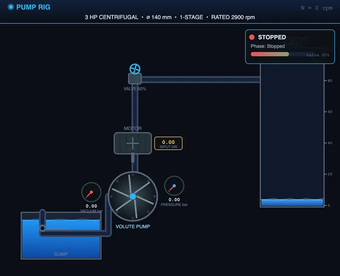
A centrifugal pump test rig measures how a pump's head, power and efficiency change with discharge. You throttle the delivery valve at constant speed and record head, flow and input power at each step, then plot the three characteristic curves against discharge and read the best efficiency point off the efficiency peak.
This virtual rig runs that experiment. The delivery valve sets the resistance of the system, and the discharge is solved as the intersection of the pump curve with the system curve — so raising the static lift really does cut the flow, and closing the gate really does walk the operating point up the H–Q curve. It also applies the affinity laws for variable speed, and checks NPSH against cavitation with live altitude and water-temperature controls. Every reading is computed from first principles, in line with IS 9137 and ISO 9906 acceptance-test practice.
When I first ran a real pump test, what surprised me was how flat the efficiency curve is on either side of the BEP. The textbook curve looks like a sharp peak; the actual measurement is closer to a gentle dome — useful, because it means you don't lose much by running a little off-design, but also a trap, because that flatness hides the start of cavitation and recirculation losses.
Centrifugal Pump Test Rig — Parameters at a Glance
| Parameter | Symbol | Range in this rig | What it changes |
|---|---|---|---|
| Pump speed | N | 800–3500 rpm | H ∝ N², Q ∝ N, P ∝ N³ (affinity laws) |
| Delivery valve opening | v | 0–100 % open | System resistance k ∝ (100/v)³; the flow follows |
| Impeller diameter | D | 90–260 mm | H ∝ D², Q ∝ D (trim laws) |
| Number of stages | — | 1–6 | Multiplies head; discharge unchanged |
| Static suction lift | hₛ | 0–7 m | Raises the system curve and lowers NPSH available |
| Static delivery lift | hₒ | 0–40 m | Raises the system curve only |
| Site altitude | z | 0–4000 m | Lowers pₐₜₘ: 101.3 kPa at sea level, 70.1 kPa at 3000 m |
| Water temperature | T | 5–95 °C | Raises p: 2.34 kPa at 20 °C, 47.4 kPa at 80 °C |
| Shut-off head | H₀ | read-out | Head at zero flow, gate closed |
| Shut-off shaft power | P₀ | read-out | ρgQ₋ₑₚH₀/(2ηₘₐₓ) — about 71 % of the BEP power |
| Specific speed | Nₛ | read-out | N√Q/H3/4 at the BEP, per stage |
What Are the Characteristic Curves of a Centrifugal Pump?
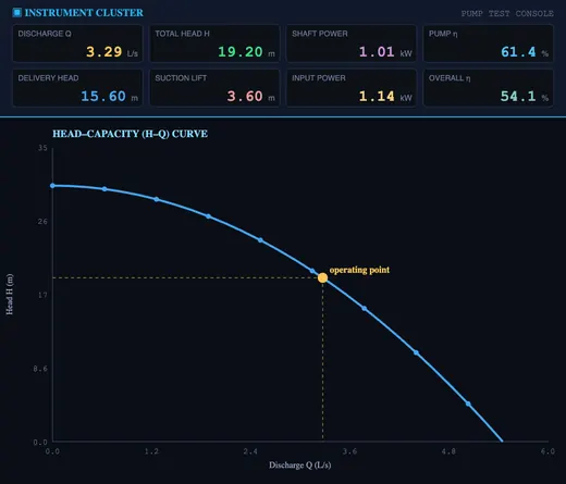
Three curves, all plotted against discharge Q at a fixed speed. The head-capacity (H–Q) curve falls as the flow rises, starting at the shut-off head with the gate closed. The shaft-power curve rises with flow from a finite shut-off value. The efficiency curve rises to a peak at the BEP and falls away on both sides. The total head is read from the suction and delivery gauges as H = (pₒ − pₛ)/ρg plus the gauge datum and the velocity-head difference.
A bench can only measure out to the flow it reaches with the gate wide open — free delivery needs an installation with no static lift and no pipe friction, which nothing real has. That is why this simulator draws the measurable part of the H–Q curve solid and the extrapolation beyond it faint, exactly as a manufacturer's published curve stops at its last measured point.
How Do You Find the Best Efficiency Point of a Pump?
Run the constant-speed test and read it off the efficiency peak. The water (output) power is Pₒ = ρgQH; it is zero at shut-off and at free delivery and peaks in between. The efficiency — water power over shaft power — is therefore zero at both ends and maximum somewhere between: that maximum is the best efficiency point, and the head and flow at it are the pump's rated duty.
The shaft power, by contrast, does not start at zero. Both Pₒ and the efficiency vanish in proportion to Q as the gate closes, so their ratio has a real limit: P_shaft(0) = ρgQ₋ₑₚH₀/(2ηₘₐₓ), which for a pump with the usual 30 % head droop works out at about 73 % of the BEP power once the flow it still churns round the wear ring is counted. A power curve drawn diving to zero at Q = 0 is a modelling artefact — the impeller is still churning water round the casing, and the motor still feels it. Running close to the BEP minimises energy cost, vibration and wear; the lab test exists precisely to find that point.
Why Doesn’t the Duty Point Follow the Affinity Laws?
Because the affinity laws scale the pump curve, not the operating point. The laws say discharge varies as N, head as N² and power as N³ for a fixed impeller, and that is exactly true of the curve itself. But the duty point is where that curve crosses the system curve, H = Hₛₜₐₜₛₓ + kQ² — and the static head does not shrink when you slow the pump down. Slow the machine and the duty point drifts off the affinity prediction, always toward less flow than Q ∝ N promises.
On a purely friction system, with no static lift at all, the two coincide exactly — set both static lifts to zero in Pump Setup and the gap closes. This is the practical limit on sizing a variable-speed drive from the affinity laws alone, and the Variable-Speed test plots the measured duty points against the prediction so the divergence is visible rather than assumed. The specific speed Nₛ = N√Q/H⁹⃗⁷⁵, evaluated at the BEP per stage, classifies the impeller as radial, mixed or axial flow and lets pumps of different sizes be compared.
What Is NPSH, and When Does a Pump Cavitate?
If the pressure at the impeller eye falls to the liquid's vapour pressure, the liquid boils and cavitation begins — collapsing vapour bubbles erode the impeller, the pump makes a noise like gravel going through it, and the head and efficiency drop sharply. The available margin is the net positive suction head, NPSHₐ = (pₐₜₘ − pₙ)/ρg − suction lift − suction friction, and it must stay above the pump's required NPSH, which rises with the square of discharge.
Three things eat the margin, and all three are live controls here. Altitude: the atmosphere pushes with 101.3 kPa at sea level but only 70.1 kPa at 3000 m, worth 3.2 m of NPSHₐ. Temperature: water's vapour pressure is 2.34 kPa at 20 °C and 47.4 kPa at 80 °C, worth another 4.5 m. Flow: suction friction and NPSHₕ both grow as Q². A pump perfectly happy at sea level on cold water can cavitate on the same duty in a hot country up a hill — and in this rig it will, with the head visibly breaking down and vapour bubbles at the impeller eye. Note that NPSHₕ belongs to the first-stage impeller alone, so on a multistage pump it scales with the head per stage, not the total.
How Do You Diagnose a Worn Centrifugal Pump?
By separating the losses. Overall pump efficiency is the product of three: ηvol (how much of what the impeller pumps actually leaves the discharge), ηhyd (how much of the impeller's work survives friction and shock inside the waterway) and ηmech (bearings, seal faces, coupling). Each defect attacks a named term, so the breakdown tells you where to look: a falling ηvol means clearances, a falling ηhyd means surfaces, a falling ηmech means the drive train.
The wear ring is the usual first casualty. It is a renewable annular clearance at the impeller eye; API 610 sets the diametral clearance when new, and industry renews the rings once the measured clearance reaches about twice that — the "2× rule". Leakage through the ring is an annular orifice, proportional to the clearance and to √H, so each doubling costs 3–5 efficiency points and raises NPSH required by roughly 50 %: the leakage jet re-entering the eye disturbs the inlet flow, which is the mechanism behind both numbers.
Vibration completes the picture, because each fault stands at its own frequency. Unbalance sits at 1× shaft speed; misalignment at 2×; blade–tongue interaction at the vane-pass frequency, vanes × shaft speed. A rolling-element bearing generates four frequencies from its geometry alone — BPFO on the outer race, BPFI on the inner, BSF on a rolling element, FTF for the cage — and none is a whole number of shaft orders, which is precisely why a bearing fault can be told apart from a rotor fault. An inner-race defect rotates in and out of the load zone once per revolution, so BPFI carries sidebands one shaft order apart; an outer-race defect, stationary in the load zone, does not. Cavitation has no line at all: it lifts the broadband floor, and that absence is the diagnosis.
The verdict comes from ISO 10816-7, the rotodynamic-pump part of the machine-vibration standard. For a general-service pump under 200 kW, zone A is ≤ 3.2 mm/s RMS (newly commissioned), zone B ≤ 5.1 (unrestricted long-term operation), zone C ≤ 8.5 (unsatisfactory — plan remedial work) and zone D above that. Reliability studies put bearings at roughly 45 % of centrifugal pump failures and mechanical seals at about 30 %, though seals are often the symptom rather than the cause.
Who Uses This Simulator?
Mechanical, civil and chemical engineering students use this rig in fluid machinery, hydraulics and turbomachinery labs; diploma and vocational students use it to learn pump performance testing without a physical bench; and instructors use it to demonstrate the BEP, affinity laws and cavitation safely and repeatably. It is built for BTech, polytechnic and AMIE fluid-machinery courses.
Explore Related Simulators
Continue exploring fluid machinery and lab-testing tools on MechSimulator. Compare the pump bench with the Hydraulic Turbine Test Rig (a pump is essentially a turbine run in reverse), the IC Engine & Morse Test Rig for performance-curve and efficiency testing of a prime mover, study the Centrifugal Governor for speed control of rotating machines, see flow-regime transition in the Reynolds Number simulator, and apply the Continuity Equation to relate pipe velocity and discharge.
Updated