Reynolds Number Simulator & Virtual Lab
Re = ρvD / μ — Osborne Reynolds’ dye experiment, live • Laminar vs Turbulent • Simulate • Explore • Practice • Quiz
Display Controls
Σ Live equations — values substituted
⚖ Fluid comparison — Re for current v & D
💡 What-if coach — insights
1 Overview
The Reynolds Number Simulator is the simplest visual answer to one of fluid mechanics’ most important questions: is this flow laminar or turbulent? Tune the velocity, pipe diameter, and fluid, and watch the particle paths morph from neatly parallel streamlines (laminar) to chaotic eddies (turbulent) as the live Re reading crosses 2300.
Six fluids are pre-loaded spanning seven decades of viscosity — from air (μ = 1.81×10⁻⁵ Pa·s) and water through oil and glycerin to honey (μ ≈ 10 Pa·s). Built for high-school and technical-college fluid-mechanics introductions, with Practice and Quiz modes for self-testing.
2 Configuring the System

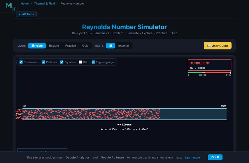
The simulator opens with water at 20 °C flowing at 2 m/s through a 4 cm diameter pipe — Re ≈ 80 000, well into turbulent. Watch the tracers tumble through the pipe and the injected dye filament burst into eddies. Bring the velocity down below 0.058 m/s and Re falls under 2300; the tracers slow, the profile opens into a parabola, and the dye straightens into a single line the whole length of the run.
Try the Honey Pour preset — even at 1 m/s through a 5 cm pipe, Re is only ~700: pure laminar flow no matter what. Then switch to the Tap Water preset for tens of thousands. The regime gauge at top right shifts through green (laminar), gold (transitional), and red (turbulent).
The View switch under the canvas chooses the picture. Real (the default) draws the experiment as it stands in a teaching lab: a constant-head tank whose level is held by an overflow standpipe, a dye reservoir and needle feeding the bell-mouth on the centreline, the glass test tube on saddle posts, and a control valve discharging into a measuring cylinder. The cylinder fills at the true flow rate, and the plate beside it shows the time, the volume collected and Q = V/t — the way Reynolds’ apparatus is actually read. Air runs through the same tube as a smoke rig with a suction fan, and the flat plate sits in a bench-top flume. Diagram shows the pipe alone with the diameter ruler. The fittings around the tube are not to scale; the tube’s length is (see the scale bar).
3 Running the Cycle
Adjust Velocity (0.01–10 m/s) and Diameter (0.1–30 cm), set the Temperature, pick a fluid and a duct shape, and read the live Re value on the canvas and in the readout cards. The particle pattern updates immediately — smooth parallel for laminar, mixed weave for transitional, full chaotic eddies for turbulent.
Every tracer moves at the true local velocity for its position in the pipe, not at some average, which is why the flow looks different either side of the transition. Below Re 2300 the profile is the Hagen–Poiseuille parabola, so the centreline runs at exactly twice the mean velocity and the particles visibly shear past one another. Above Re 4000 the profile is the power law u/umax = (1 − r/R)1/n, whose exponent is read from the standard table (n = 6.0 at Re = 4×10³ rising to 10 at 3.2×10⁶); at n = 7 the centreline runs at 1.22 times the mean, so the flow moves almost as a plug with the shear squeezed into a thin layer at the wall. Both profiles integrate to exactly the mean velocity you dialled in. Hover or tap anywhere in the bore to read r/R, the local u and u/umax at that radius.
The red thread is Osborne Reynolds’ dye filament — the 1883 experiment this number is named after. A needle injects dye on the centreline at the inlet. In laminar flow it stays a razor-straight line the whole length of the pipe; through the transition it wavers and begins to break up a few diameters downstream; in turbulent flow it bursts into eddies and smears across the bore. That lag before break-up is real, and it is what makes “transitional” look different from “turbulent” rather than merely noisier.
Two notes on how to read the canvas. The animation runs in slow motion at a stated fraction of real time (the note under the scale bar says which), so the flow is watchable at 10 m/s as well as at 1 cm/s; changing the playback speed changes only the clock, never the physics. And the turbulent eddying is drawn with a stated visual gain, because the real turbulence intensity — printed on the gauge as I = 0.16 Re−1/8, a few per cent — would be invisible at this size. Bore diameter is compressed by default so a 1 mm capillary and a 300 mm main are both legible; untick Fit small bores for a true 1:1 scale.
Ten readout cards report Re, regime, ρ, μ, ν, volumetric flow rate Q, the critical velocity for the current diameter (where Re = 2300), the Darcy friction factor, the hydrodynamic entrance length, and the hydraulic diameter. The last four are relabelled when you switch to external flow, because the same slots then mean plate length, skin friction, transition location and boundary-layer thickness. + Custom lets you add your own fluid with a user-defined density and dynamic viscosity.
Temperature. Viscosity is the biggest real-world lever on Reynolds number, and the temperature control moves it. Where a standard correlation exists it is used — water from μ = 2.414×10−5·10247.8/(T−140) with Kell’s density polynomial, air from Sutherland’s law with density from the ideal gas law — and glycerin and mercury are interpolated from published tables, in log space, because viscosity falls roughly exponentially with temperature. Vegetable oil and honey are held at their reference temperature and the control greys out: both are variable natural products with no standard correlation, and an invented fit would be worse than an absent feature. The effect is not subtle. Heating glycerin in a 4 cm pipe at 2 m/s from 20 °C to 100 °C takes Re from 71 to 6550 — laminar, through transitional, to turbulent — without touching velocity or diameter. That is why oil pipelines are heated and why a cold engine is harder to turn over.
Duct shape. Re is not a pipe-only number. For any non-circular duct the characteristic length is the hydraulic diameter Dₕ = 4A/P, which is generally not a width you can measure with a rule: a 4:1 rectangular duct 4 cm tall has Dₕ = 6.4 cm. The shape selector switches between a round pipe, square, 2:1, 4:1 and 8:1 rectangular ducts, and the parallel-plate limit; the size control always sets the short cross-section dimension and Dₕ is derived from it, so the cross-section drawn beside the duct shows exactly where the number comes from. It also corrects the friction factor: f = 64/Re is the circular case only. The Poiseuille number f·Re runs from 56.92 for a square duct through 64 for a pipe to 96 between parallel plates — a 1.7× spread that the single familiar formula hides. A square duct and a round pipe of the same height have the same Dₕ and the same Re, and still do not have the same friction.
External flow. Choosing Flat plate changes the problem, not just the picture. Over a surface the characteristic length is the distance from the leading edge, so Re grows along the plate and the flow trips part way along rather than all at once — and it trips at Reₓ ≈ 5×10⁵, more than two hundred times the pipe’s 2300. The canvas draws the boundary layer growing from the leading edge (δ = 5x/√Reₓ while laminar, 0.37x/Reₓ1/5 once turbulent), marks where it transitions, and reports the average skin-friction coefficient in place of the Darcy factor. Note the regime gauge: the same axis, with the green band now running out to 5×10⁵. The vertical scale is exaggerated four times and the canvas says so, because a real boundary layer is a couple of per cent of the plate length — on a 30 cm plate in water at 2 m/s it is about 2.5 mm.
Two of those cards deserve a note. The friction factor quoted is the smooth-pipe value: 64/Re while laminar, which is exact, and the Colebrook relation at zero roughness above the transition. Through the transitional band itself it is marked with a ?, because no single friction factor is valid there — the flow is intermittent, and the honest answer is a range. Real pipes are not smooth, and the roughness ratio ε/D can easily double f; for the Moody chart, the Colebrook solution with roughness and the resulting head loss, use the Fluid Flow simulator, which is built for exactly that.
The entrance length Lₑ is the length of straight pipe the flow needs before the velocity profile drawn on the canvas actually exists, measured from the inlet: Lₑ = 0.05 Re D while laminar, and about 1.36 D Re1/4 once turbulent. The two agree near the transition — that formula gives about 11 diameters at Re = 4000, which is where the familiar “ten diameters” rule of thumb comes from — but they part company higher up, where it grows to roughly 40 diameters, so the ten-diameter shortcut is optimistic for fast flow. A dashed marker on the pipe shows where it falls. This matters more than it sounds: water creeping at 0.05 m/s through a 4 cm pipe needs 4 m of straight run to develop, so in the 1 m length drawn the profile is still forming the whole way. When Lₑ exceeds the run shown, the note under the scale bar says so rather than letting the picture imply otherwise. It is also why fittings, bends and instruments need a straight approach: put a flow meter five diameters after an elbow and it reads a profile that has not settled.
4 The Underlying Theory
Switch to Explore for concept cards in four categories. Basics covers what laminar and turbulent flow are physically, why viscosity matters, and the dimensionless-number idea. Formulas derives Re, kinematic viscosity, and the connection to friction factor. Applications covers pipelines, blood flow, aircraft wings, and microchannels. Common Errors warns about unit traps, characteristic-length confusion, and assuming Re = 2300 for non-pipe geometries.
5 Try a Problem
Practice gives randomised problems — compute Re for given v, D, fluid; find the critical velocity for laminar-turbulent transition; rearrange to find diameter or velocity. Tolerance ~5%. Show Solution walks through every step.
Quiz presents five mixed conceptual + numerical questions per session including identifying flow regime from Re, predicting the effect of changing v or D, and applying the formula in real-world contexts.
6 Engineering Notes
- Re scales with v and D linearly — halving D halves Re, doubling v doubles Re.
- Re scales inversely with viscosity, so honey (μ ~ 10 Pa·s) is virtually impossible to make turbulent at human scales.
- The 2300 threshold applies to fully-developed pipe flow. Open-channel and external flow have different transition Reynolds numbers.
- For the same density and viscosity, kinematic viscosity ν = μ/ρ is what really matters for Re — mercury has high μ but also high ρ, so its ν is moderate.
- Pair this with the Fluid Flow in Pipes, Bernoulli’s Principle, and Wind Tunnel for more dynamics practice.
Understanding the Reynolds Number and Flow Regimes
The Reynolds number (Re) is a dimensionless ratio of inertial forces to viscous forces in a flowing fluid. It is the single most important parameter for predicting whether a flow is laminar (orderly) or turbulent (chaotic). The formula is Re = ρvD / μ, where ρ is fluid density, v is mean velocity, D is the characteristic length (pipe diameter), and μ is dynamic viscosity.
Properties of Common Fluids
| Fluid | ρ (kg/m³) | μ (Pa·s) | ν (m²/s) | Re at v = 1 m/s, D = 5 cm |
|---|---|---|---|---|
| Air (20°C) | 1.20 | 1.81×10⁻⁵ | 1.51×10⁻⁵ | 3 313 |
| Water (20°C) | 1000 | 1.00×10⁻³ | 1.00×10⁻⁶ | 50 000 |
| Mercury | 13 534 | 1.55×10⁻³ | 1.15×10⁻⁷ | 437 000 |
| Vegetable oil | 920 | 0.084 | 9.13×10⁻⁵ | 548 |
| Glycerin | 1260 | 1.412 | 1.12×10⁻³ | 44.6 |
| Honey (20°C) | 1420 | 10.0 | 7.04×10⁻³ | 7.10 |
Flow Regimes for Pipe Flow
For fully-developed flow inside a circular pipe, three regimes are conventional: laminar (Re < 2300), transitional (2300 ≤ Re ≤ 4000), and turbulent (Re > 4000). Laminar flow has a smooth parabolic velocity profile and low friction; turbulent flow has a flatter profile and much higher friction. The transition is not razor-sharp — it depends on inlet conditions, surface roughness, and disturbances — but 2300 is a reliable engineering rule of thumb.
Why Viscosity Dominates Small-Scale Flow
Halving D or v halves Re. Inversely, multiplying viscosity by 10 divides Re by 10. This is why honey, syrup, and oil almost always flow laminar at human scales — viscosity dwarfs inertia. It is also why microfluidics (lab-on-chip devices with channels under 100 μm) are inherently laminar: D is so small that Re stays well below 1, and the only way to mix two streams is by diffusion or careful geometry.
Engineering Applications
The Reynolds number governs design in nearly every fluid-handling system. Pipelines are sized so that flow is comfortably turbulent for good mixing and heat transfer, while keeping pumping costs reasonable. Aircraft wings use a chord-based Re — whether the boundary layer is laminar or turbulent affects lift and drag dramatically. Blood flow in the aorta sits at Re ≈ 4000 (top of the transitional range), while capillaries are deeply laminar. Heat exchangers exploit turbulent flow for vastly better heat transfer than laminar.
The Critical Velocity
For a given fluid and pipe diameter, the critical velocity is the speed at which Re crosses 2300: vcrit = 2300 · μ / (ρ · D). Below vcrit the flow is laminar; above, it transitions to turbulent. For water in a 1 cm pipe, vcrit ≈ 0.23 m/s — even a slow water tap is already turbulent. For honey in the same pipe, vcrit would need to be > 1600 m/s — physically impossible.
Why “Inertia vs Viscosity” Actually Makes Sense
The standard textbook line is that Re is a ratio of inertial forces to viscous forces. That is true but unsatisfying. The intuition: how much does a parcel of fluid resist being deflected (inertia, depends on momentum ρv) compared to how much the surrounding fluid drags on it sideways (viscous, depends on shear gradient μv/D)? When inertia dominates, a perturbation grows into a swirl — you get turbulence. When viscosity dominates, perturbations damp out — you get laminar flow. Re is just the cleanest dimensionless way to write that ratio.
The same dimensionless ratio shows up everywhere: aircraft wings (where D is wing chord), insect flight (Re ~100, deeply laminar, requires totally different aerodynamics from aircraft), bacterial swimming (Re ~10−4, “swimming in tar” as Edward Purcell put it), even stirred coffee (Re ~105, fully turbulent, which is why the milk and coffee mix in seconds).
Three Specific Calculations Worth Internalising
| Scenario | Re | Regime |
|---|---|---|
| Water from a tap, 10 mm pipe, 1 m/s | 1000×1×0.01/10−3 = 10,000 | Turbulent |
| Honey through the same pipe at the same speed | 1420×1×0.01/10 = 1.4 | Deeply laminar |
| Blood in the aorta, 25 mm diameter, 0.5 m/s | 1060×0.5×0.025/3.5×10−3 = 3800 | Top of transitional |
| Air at the wingtip of a 747 cruising at 250 m/s, 6 m chord | 0.4×250×6/1.4×10−5 = 4.3×10⁷ | Deep turbulent |
| A bacterium swimming at 30 µm/s in water | 1000×3×10−5×2×10−6/10−3 = 6×10⁻⁵ | Stokes (creeping) flow |
Notice the range: from 10−5 for a bacterium to 107 for an airliner. Twelve orders of magnitude. The same physical equations describe both, with Re as the parameter that controls which regime you’re in.
When the 2300/4000 Boundary Lies to You
Those textbook numbers are for an idealised case: long straight smooth pipes with carefully controlled inlet. Real engineering pipes rarely meet that ideal:
- Disturbed inlet. A 90° elbow or sudden contraction injects turbulence into otherwise laminar flow. Transition may start as low as Re ~1500.
- Carefully smooth inlet. Reynolds himself, with a flared bell-mouth entry and very smooth pipe, kept laminar flow up to Re ~13,000 in lab experiments. The textbook 2300 is conservative.
- Pipe roughness. Rough pipes destabilise laminar flow earlier and produce fully-turbulent flow at lower Re than smooth pipes.
- Curved pipes (coiled tube reactors). Curvature stabilises laminar flow through Dean vortices. Transition can be delayed to Re > 10,000.
Osborne Reynolds’ Dye Experiment, Recreated
The number is named after the 1883 experiment, and this simulator runs it. A needle injects a dye filament on the centreline at the inlet, exactly as Reynolds did with coloured water in a glass tube. Below Re 2300 the thread stays a razor-straight line the whole length of the pipe — that is what “direct motion” meant in his title. Through the transition it wavers, then breaks up a few diameters downstream. Above Re 4000 it bursts into eddies within a short distance of the needle and smears across the bore. That lag before break-up is real and it is the part most textbook diagrams omit: transition happens at a place along the pipe, not everywhere at once.
Reynolds’ own apparatus reached laminar flow up to Re ≈ 13,000 with a flared bell-mouth entry, which is why the 2300 figure is a conservative engineering rule rather than a law of nature. Use the temperature control to reproduce the other half of his insight: warming the water lowers μ, raises Re at fixed velocity, and trips the filament without touching the tap.
Hydraulic Diameter: Reynolds Number for Non-Circular Ducts
Re = ρvD/μ needs a characteristic length, and for anything that is not a round pipe that length is the hydraulic diameter Dₕ = 4A/P — four times the flow area divided by the wetted perimeter. It is generally not a dimension you can measure with a rule. A rectangular duct 4 cm tall with a 4:1 aspect ratio has Dₕ = 6.4 cm, so at the same air speed its Reynolds number is 60 % higher than a 4 cm pipe’s. Between parallel plates a gap b gives Dₕ = 2b.
The same correction applies to friction, and it catches people out: f = 64/Re is the circular case only. The Poiseuille number f·Re is a property of the cross-section — 56.92 for a square duct, 64 for a round pipe, 96 between parallel plates. That is a 1.7× spread hidden inside one familiar formula. Select any shape in the simulator and the cross-section is drawn to scale beside the duct with 4A/P spelled out.
Entrance Length: When the Profile Is Not Developed Yet
Every textbook Reynolds calculation assumes fully-developed flow, and almost nobody checks whether the pipe is long enough for that to be true. The hydrodynamic entrance length is Lₑ = 0.05 Re Dₕ while laminar and about 1.36 Dₕ Re1/4 once turbulent. Water creeping at 0.05 m/s through a 4 cm pipe needs 4 metres of straight run before the parabola exists; vegetable oil at 1 m/s in a 10 cm pipe needs 5.5 m.
This is why instruments have straight-run requirements. Put an orifice plate or a flow meter five diameters after an elbow and it reads a profile that has not settled, and the calibration — which assumed a developed profile — is simply wrong. The simulator marks Lₑ on the pipe and tells you when it exceeds the length being drawn.
Re Beyond Pipes: Flat Plates and Boundary Layers
The 2300 threshold is a pipe number. Switch the simulator to Flat plate and the problem changes: the characteristic length is the distance x from the leading edge, so Re grows along the surface and the flow trips part way along rather than all at once. Transition sits at Reₓ ≈ 5×10⁵ — more than two hundred times the pipe value. Open channels transition around 500; a sphere’s drag crisis happens near 3×10⁵. The number is universal; its critical value is not.
The boundary layer grows as δ = 5x/√Reₓ while laminar and 0.37x/Reₓ1/5 once turbulent, and the simulator draws it with the transition point marked. On a 30 cm plate in water at 2 m/s the layer is only about 2.5 mm thick at the trailing edge — a couple of per cent of the plate length, which is why the vertical scale on that view is exaggerated and labelled as such.
Viscosity Is Where Temperature Hides
Density barely moves with temperature; viscosity moves enormously, and Re depends on their ratio. Glycerin at 20 °C has μ = 1.412 Pa·s; at 100 °C it is 0.0148 — a factor of 95. Run the simulator at 2 m/s in a 4 cm pipe and heating the glycerin alone takes Re from 71 to 6550, carrying the flow from deeply laminar, through the transitional band, into turbulence without touching the velocity or the pipe.
That single effect explains heated crude-oil pipelines, why a cold engine is harder to turn over, and why a viscosity figure quoted without a temperature is useless. Water and air here follow standard correlations; glycerin and mercury are interpolated from published tables. Vegetable oil and honey are held at 20 °C and the control greys out, because neither has a standard viscosity–temperature correlation and an invented one would be worse than none.
References
- Reynolds, O. (1883) — An experimental investigation of the circumstances which determine whether the motion of water shall be direct or sinuous. Phil. Trans.
- Purcell, E. M. (1977) — Life at low Reynolds number. Am. J. Phys. 45, 3. A classic, short, beautifully written paper.
- White, F. M. — Fluid Mechanics, 8th ed., Chapter 6.
Explore Related Simulators
If you found this Reynolds number simulator helpful, explore our Viscosity Experiment Virtual Lab, Continuity Equation, Fluid Flow in Pipes, Bernoulli’s Principle, Wind Tunnel, Airfoil Calculator, Pascal’s Law, the Centrifugal Pump Test Rig, and the Hydraulic Turbine Test Rig for more practice. The Orifice Experiment Virtual Lab shows why the regime matters: below Re ≈ 104 the tabulated discharge coefficients stop applying.
Updated
Density 100–15 000 kg/m³. Viscosity 1e-6 to 100 Pa·s.