Continuity Equation Simulator
A₁V₁ = A₂V₂ — Mass conservation in flow • Simulate • Explore • Practice • Quiz
Display Controls
Σ Live equations — values substituted
⚖ Section comparison — areas, velocities, Q
💡 What-if coach — insights
1 Overview
The Continuity Equation Simulator visualises the fundamental conservation of mass in incompressible flow: A₁·V₁ = A₂·V₂. A horizontal pipe changes cross-section between two sections. Where the pipe narrows, the fluid must speed up to keep the volumetric flow rate Q constant; where it widens, the fluid slows down by the same rule.
Adjust three sliders — D₁ (inlet), D₂ (outlet), and V₁ — and watch V₂ jump as the geometry changes. Built for high-school and technical-college physics, with Practice and Quiz modes for self-testing.
2 Configuring the System

Defaults: D₁ = 10 cm, D₂ = 5 cm, V₁ = 2 m/s. Halving the diameter quarters the area, so V₂ = 4×V₁ = 8 m/s. Try the Garden Hose Nozzle preset to see a 5× speed-up. D₂ may also be set larger than D₁ — the Diffuser (Expansion) preset shows the inverse case, where the same Q spread over a wider area means the fluid slows down.
3 Running the Cycle
Tracer particles travel left-to-right at the true local velocity — the on-screen speed is directly proportional to V, so doubling V₁ visibly doubles how fast the flow moves. They ride fixed streamtubes, so they converge through the contraction exactly as the streamlines do. Both velocity arrows are drawn to one shared scale, so the arrow at section 2 is literally V₂/V₁ times longer than the one at section 1.
A violet fluid parcel is released at the inlet every so often. It always carries the same volume, so as it enters the narrow section it stretches lengthwise by exactly the same factor that its cross-section shrinks — the clearest single picture of A·V = constant. Hover or tap anywhere along the pipe to place a cross-section probe: it reads D, A and V at that station and shows Q = A·V, which never changes from inlet to outlet.
The panel at the bottom-left carries the equation in its ratio form, A₁/A₂ = V₂/V₁, with the live values substituted underneath — so the area ratio and the velocity ratio are always shown to be the same number. The colours are crossed deliberately: section 1 is cyan and section 2 amber, so on the left the cyan term is on top and on the right the amber one is, which is the inversion the equation is about. Both sides are ratios and therefore dimensionless; the units stay on the captions beside the pipe, and Q is printed above both sections.
A ruler at the left gives the vertical (diameter) scale, and both sections are measured against that one ruler. By default the view is fitted: the pipe is enlarged so that small-bore cases such as the garden hose stay readable, which means the vertical scale steps down as the larger diameter grows. Turn Zoom to fit off for a single fixed scale (marked 1:1) across the whole slider range — then each diameter slider moves only its own section, and a 1.6 cm hose really is drawn 19× smaller than a 30 cm culvert. Either way the two sections always keep their true ratio, and the D and A readouts are unaffected by the view setting.
The fluid tint maps to speed (blue = slow, amber = fast) against the legend at the bottom-right, and the scale bar gives the pipe's physical length. The animation runs at a fixed fraction of real time (shown on the canvas); use the Speed selector in Display Controls to slow it to 0.25× or run it at 4× — this changes only the playback rate, never the physics. Live readouts show A₁, A₂, V₁, V₂, Q, and the ratio V₂/V₁ = (D₁/D₂)². Seven presets cover hoses, blood vessels, river constrictions, wind tunnels and a diverging diffuser.
4 The Underlying Theory
Four categories: Basics (mass conservation, incompressibility), Formulas (deriving A·V = const, Q = A·V), Applications (hose, aorta, river, wind tunnel, dam spillway), Common Errors (radius vs diameter, units, compressible flow).
5 Try a Problem
Practice generates problems — find V₂ given A₁, A₂, V₁; find required D₂ for a target speed-up; identify Q given any pair. Quiz tests conceptual + numerical with 5 questions.
6 Engineering Notes
- Velocity scales with the inverse square of diameter, not directly with diameter.
- The continuity equation only applies to incompressible flow (liquids, low-speed gases). Above ~Mach 0.3, density changes break the assumption.
- Q is conserved everywhere along a single pipe with no branches. With branches, Q in = sum of Q out.
- Pair this with the Bernoulli’s Principle simulator — pressure drops where velocity increases.
- Pair with the Reynolds Number simulator to check the flow regime.
Understanding the Continuity Equation
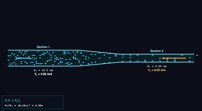
The continuity equation expresses conservation of mass for fluid flow. For an incompressible fluid (constant density ρ), the volumetric flow rate Q = A·V must be the same at every cross-section of a pipe with no branches: A₁·V₁ = A₂·V₂. Where the pipe is narrower, the fluid must move faster to deliver the same volume per second.
The V ∝ 1/D² Rule
| D₂/D₁ | A₂/A₁ | V₂/V₁ | Example |
|---|---|---|---|
| 1.0 | 1.00 | 1.0× | Constant pipe |
| 0.71 | 0.50 | 2.0× | Half-area constriction |
| 0.50 | 0.25 | 4.0× | Default sim |
| 0.33 | 0.11 | 9.0× | Hose with thumb partly over end |
| 0.20 | 0.04 | 25× | Spray nozzle |
| 0.10 | 0.01 | 100× | Fire-hose tip |
Garden Hose vs Aorta
Pinching a garden hose with your thumb is the most everyday demonstration of A·V = const. Reducing the open area by 4× quadruples the exit velocity, sending water much further. The same physics gives a fire hose its long throw — high pressure pumps water through a wide hose, but the narrow nozzle at the end does the speed-up. In your body, the aorta (D ≈ 2.5 cm) carries blood at v ≈ 30 cm/s. By the time blood reaches the capillaries (D ≈ 8 μm, but billions of them in parallel), the total cross-sectional area is >1000× larger and average velocity drops to <1 mm/s — ideal for slow gas exchange.
Volumetric vs Mass Flow Rate
For incompressible flow, volumetric flow rate Q = A·V is conserved. For compressible flow (gases at high speed, hot gas in turbines), it’s the mass flow rate ρ·A·V that’s conserved — density changes too, and the geometry-velocity relationship is different. The continuity equation for compressible flow becomes ρ₁·A₁·V₁ = ρ₂·A₂·V₂.
Continuity in Engineering
Engineers use continuity in pipe sizing, nozzle design, fan and pump selection, ventilation ducting, blood-flow modelling, and stream-flow predictions in environmental engineering. Combined with Bernoulli’s principle (which tells you how pressure changes with velocity), continuity gives you the basics for designing every fluid-handling system — from a simple garden hose to a turbojet engine.
Who Uses This Simulator?
Used by high-school physics students learning conservation laws, technical-college trainees in fluid mechanics, biomedical engineering students analysing circulatory flow, and HVAC trainees sizing ducts. Practice and Quiz modes ensure students can apply the formula to varied scenarios.
Explore Related Simulators
If you found this continuity equation simulator helpful, explore our Bernoulli’s Principle, Reynolds Number, Fluid Flow in Pipes, Pascal’s Law, Wind Tunnel, the Centrifugal Pump Test Rig, and the Hydraulic Turbine Test Rig for more practice. The Orifice Experiment Virtual Lab applies the same A×V bookkeeping to a contracting jet, where the area at the vena contracta is what the coefficient of contraction measures.
Updated