Heat Transfer Simulation: Conduction, Convection & Radiation
Conduction • Convection • Radiation — Simulate • Explore • Practice • Quiz

1 Overview
The SI / Imperial switch in the mode bar restates all three modes in US/IP heat-transfer units (Btu/hr, Btu/hr·ft², °F, ft², inches). ΔT converts with the 1.8 factor and no 32° offset, since it is a difference.
The Heat Transfer Modes Simulator covers the three fundamental mechanisms by which thermal energy moves: conduction (through solid materials, governed by Fourier's Law), convection (between a surface and a moving fluid, governed by Newton's Law of Cooling), and radiation (through electromagnetic waves, governed by the Stefan-Boltzmann Law). Each mode has its own set of controls, formulas, and visualisations.
This simulator is designed for mechanical engineering students studying heat transfer, thermal systems designers, HVAC engineers, and instructors teaching thermal resistance, heat flux, and temperature gradient concepts. The four interactive modes — Simulate, Explore, Practice, and Quiz — provide a complete learning pathway from visual experimentation to self-assessment.
2 Configuring the System

The simulator opens in Simulate mode with Conduction selected. You see a steel wall with Thot = 400 °C on one side and Tcold = 50 °C on the other. The canvas shows an animated heat flow visualisation with a colour gradient from hot (red) to cold (blue). Readouts display the heat transfer rate Q (in watts), thermal resistance Rth, temperature gradient, heat flux, temperature difference ΔT, thermal conductivity k, the active mode, and the governing formula.
Start by switching between the three transfer modes using the Transfer Mode pill tabs. Each mode reveals its own set of controls — Conduction shows material selector and wall thickness/area/temperature sliders; Convection shows surface area, convection coefficient h, and surface/fluid temperatures; Radiation shows emissivity, area, and hot/cold body temperatures in Kelvin. The presets (Steel Wall, Brick Oven, Pipe Flow, Furnace Radiation) load realistic configurations for quick exploration.
3 Running the Cycle
In Conduction mode, the formula is Q = kAΔT/L. Choose a material (Steel k = 50, Copper k = 385, Brick k = 0.7, Glass k = 1.0 W/m·K) and adjust wall thickness, area, and the hot and cold temperatures. Watch how copper transfers far more heat than brick for the same geometry and temperatures due to its much higher thermal conductivity. The thermal resistance Rth = L/(kA) is displayed alongside the heat rate.
In Convection mode, the formula is Q = hA(Ts − T∞). Adjust the convection coefficient h (5–500 W/m²K) to simulate natural convection (low h) versus forced convection (high h). In Radiation mode, the formula is Q = εσA(T₁⁴ − T₂⁴). Adjust emissivity from 0.05 (polished metal) to 1.0 (blackbody) and observe how the fourth-power temperature dependence makes radiation dominant at high temperatures, such as in furnace applications.
4 The Underlying Theory
Switch to Explore mode to browse concept cards across three categories: Conduction, Convection, and Radiation. The Conduction category covers Fourier's Law, thermal conductivity values for common engineering materials, composite walls and series/parallel thermal resistance, and steady-state versus transient conduction.
The Convection category explains Newton's Law of Cooling, the difference between natural and forced convection, boundary layer theory, and typical h values for air, water, and oil. The Radiation category covers the Stefan-Boltzmann Law, emissivity and absorptivity, view factors, blackbody radiation, and Wien's displacement law. Each card includes formulas, worked examples, and practical engineering context to connect theory with real-world thermal design problems.
5 Try a Problem
Practice mode generates randomised heat transfer problems across all three modes. You might be asked to calculate the heat rate through a copper wall, find the convection coefficient needed to cool a surface, or determine the radiative heat exchange between two surfaces at different temperatures. Enter your answer and click Check for instant feedback. Click Next Problem to generate a new scenario.
Quiz mode presents five questions per session, mixing conceptual and numerical problems. Topics include identifying heat transfer modes, comparing thermal conductivities, calculating thermal resistance in composite walls, and solving Stefan-Boltzmann radiation problems. After completing the quiz, review your performance to identify weak areas. This mode is excellent preparation for heat transfer examinations and thermal engineering certification tests.
6 Engineering Notes
- Compare materials by switching between Steel, Copper, Brick, and Glass at the same geometry and temperatures. The enormous difference in k values (0.7 to 385 W/m·K) illustrates why material selection is critical in thermal design.
- For radiation problems, always use absolute temperature in Kelvin. The T⁴ dependence means small temperature errors produce large heat rate errors.
- The thermal resistance concept (Rth = ΔT/Q) works like electrical resistance. For composite walls, add resistances in series; for parallel paths, use the parallel resistance formula.
- Use the presets to quickly see how different engineering scenarios compare. The Furnace Radiation preset shows why radiation dominates at high temperatures (T > 500 K).
- Remember that most real engineering problems involve all three modes simultaneously. A hot pipe loses heat by conduction through insulation, convection to surrounding air, and radiation to nearby surfaces.
- Combine this simulator with the Heat Exchanger Simulator and the Thermal Expansion Calculator for a comprehensive thermal engineering study session.
Heat Transfer Modes — Conduction, Convection & Radiation

The three modes of heat transfer are conduction (Q = kAΔT/L), convection (Q = hAΔT), and radiation (Q = εσA(T1⁴−T2⁴)). Conduction occurs through solid materials, convection through fluid motion, and radiation through electromagnetic waves requiring no medium. This simulator animates all three modes with adjustable material properties.
Heat transfer is the movement of thermal energy from a region of higher temperature to a region of lower temperature. The three fundamental modes of heat transfer are conduction (through solid materials), convection (via fluid motion), and radiation (through electromagnetic waves). Understanding these mechanisms is essential for designing thermal systems, insulation, heat exchangers, furnaces, and electronic cooling.
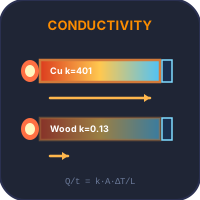
Conduction is the transfer of heat through a solid or between solids in direct contact. It is governed by Fourier’s Law: Q = kA(T1−T2)/L, where k is the thermal conductivity of the material (W/m·K), A is the cross-sectional area, L is the thickness, and (T1−T2) is the temperature difference. Metals like copper (k ≈ 385 W/m·K) conduct heat very well, while brick (k ≈ 0.7 W/m·K) is a poor conductor.
Convection — Newton’s Law of Cooling
Convection is the transfer of heat between a solid surface and a moving fluid (liquid or gas). Newton’s Law of Cooling states: Q = hA(Ts−T∞), where h is the convective heat transfer coefficient (W/m²·K), A is the surface area, Ts is the surface temperature, and T∞ is the bulk fluid temperature. Natural convection (driven by buoyancy) typically has h = 5–25 W/m²K, while forced convection (driven by fans or pumps) can reach h = 25–500 W/m²K.
Radiation — Stefan-Boltzmann Law
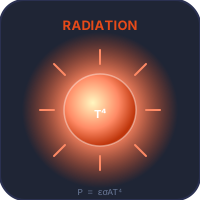
Thermal radiation is energy emitted by all bodies above absolute zero. The net radiative heat transfer between two surfaces is: Q = εσA(T14−T24), where ε is the emissivity (0–1), σ = 5.67×10⁻⁸ W/(m²·K4) is the Stefan-Boltzmann constant, and temperatures must be in Kelvin. A blackbody has ε = 1 (perfect emitter), while polished metals may have ε < 0.1.
How to Use This Simulator
In Simulate mode, select a heat transfer mode (Conduction, Convection, or Radiation), then adjust material properties and temperatures using sliders. The canvas shows an animated heat flow visualisation with temperature gradients. Readouts display heat transfer rate, thermal resistance, temperature gradient, and heat flux in real time. Use presets for common scenarios. Switch to Explore mode to study concepts across all three heat transfer modes. Practice mode generates randomised heat transfer problems, and Quiz mode tests your knowledge with 5 randomised questions.
The Kitchen Analogy — All Three Modes Around One Stove
The clearest way to feel the difference between conduction, convection and radiation is to stand near a hot pan on a gas stove. Three different mechanisms are moving heat to you at the same time.
- Conduction moves heat through the pan handle. The metal handle is solid; molecules vibrate against their neighbours and the wave of heat travels through. The handle gets uncomfortably hot in about thirty seconds. Q = kAΔT/L: a thin handle (small L) and a high-conductivity metal (large k) conduct fast. Wooden handles work because k for wood is about 1 % of k for aluminium.
- Convection heats the air above the pan and the air around you. The hot gas rises, cooler air comes in to replace it. Q = hAΔT: free convection at room temperature has h ≈ 5−25 W/m²K. Switch the fan on and forced convection raises h by ten times.
- Radiation reaches you as infrared. Even with the air still and the pan-handle in your other hand, your face feels warm. Q = εσA(T14−T24): a 500 K pan radiates 13 times more energy than a 300 K room because of the fourth-power dependence.
The three modes are always all present; one usually dominates. Engineers spend their careers figuring out which one matters in each situation and what to do about it.
A Worked Conduction Example — A 5 mm Steel Plate
A steel plate, 5 mm thick, 0.5 m by 0.5 m. One side is held at 300 °C, the other side at 100 °C. Steel has k = 50 W/m·K. How much heat flows through it?
| Step | Working | Result |
|---|---|---|
| Area | 0.5 × 0.5 | 0.25 m² |
| Temperature gradient | ΔT/L = 200 / 0.005 | 40,000 K/m |
| Heat flux | q = k·ΔT/L = 50 × 40,000 | 2 MW/m² |
| Total heat transfer rate | Q = qA = 2,000,000 × 0.25 | 500 kW |
Half a megawatt of heat through a 0.5 m square plate. Steel is good at this. Replace it with stainless steel (k ≈ 15) and the answer drops to 150 kW. Use ceramic insulation (k ≈ 0.1) and you get 1 kW. This is why oven liners are ceramic rather than steel.
When Each Mode Dominates — A Quick Sanity Check
- Inside solids. Conduction is the only mode that matters. The Fourier equation handles everything from CPU heat-sinks to building wall insulation.
- Fluid heating from a hot surface. Free convection (no fan) is usually weak; forced convection (fan or pump) is dominant. The film coefficient h is the key number, and it depends on flow speed, geometry, and fluid properties.
- Through vacuum or very still air. Radiation is the only mode that crosses. Spacecraft thermal control, vacuum-flask insulation, and the heat you feel from the sun all rely on this fact.
- Above about 600 °C. Radiation starts dominating even in air. The fourth-power scaling means a 1500 K furnace radiates 600 times more than a 500 K oven. Industrial furnaces are designed primarily as radiation devices.
Heat Transfer Simulation Online — What You Can Change and What Happens
This heat transfer simulation runs in your browser and shows all three modes with the same controls a lab would give you. Each slider changes one physical quantity, and the animation and the readouts respond together.
- Thermal conduction simulation. Raise the thermal conductivity k or shorten the wall thickness L and the temperature profile T(x) steepens, the heat flux q = kΔT/L rises and the thermal resistance R = L/(kA) falls. The profile is a straight line for a single uniform layer.
- Convection simulation. Raise the film coefficient h (free convection is about 5–25 W/m²K, forced air 25–250) and the thermal boundary layer thins, since δ ≈ k/h, so the surface loses heat faster.
- Radiation simulation. Raise the surface temperature and the emitted power climbs with T4; lower the emissivity ε and it falls in proportion. Temperatures are converted to kelvin inside the calculation.
Because every readout comes from the same equations printed in the formula table below, it doubles as a heat transfer rate calculator, a heat flux calculator and a thermal resistance calculator: set the inputs for your problem and read Q, q and R directly, then check your hand calculation against them.
Standards and References
- Cengel, Y. A. — Heat and Mass Transfer: Fundamentals and Applications, 6th ed. The clearest undergraduate treatment of the three modes.
- Incropera, F. P. — Fundamentals of Heat and Mass Transfer, 7th ed. The graduate-level reference, with deeper convection correlations.
- ASHRAE Handbook — Fundamentals chapter on Heat Transfer for HVAC-grade correlations.
- ISO 8302:1991 — Thermal insulation — Determination of steady-state thermal resistance and related properties — Guarded hot plate apparatus.
Heat Transfer Formulas — Quick Reference
| Mode | Formula | Key Variables |
|---|---|---|
| Conduction (Fourier's Law) | Q = k × A × ΔT / L | k = thermal conductivity (W/m·K), L = thickness |
| Convection (Newton's Law) | Q = h × A × (Ts − T∞) | h = convection coefficient (W/m²·K) |
| Radiation (Stefan-Boltzmann) | Q = ε × σ × A × (T1⁴ − T2⁴) | σ = 5.67 × 10−⁸ W/m²·K⁴ |
| Overall Heat Transfer | Q = U × A × ΔTlm | U = overall heat transfer coefficient |
| Thermal Resistance (wall) | R = L / (k × A) | Analogous to electrical resistance |
Thermal Conductivity of Common Engineering Materials
| Material | k (W/m·K) | Category |
|---|---|---|
| Copper | 385 | Conductor |
| Aluminium | 205 | Conductor |
| Steel (carbon) | 50 | Conductor |
| Stainless Steel (304) | 16 | Conductor |
| Glass | 1.0 | Insulator |
| Brick | 0.7 | Insulator |
| Wood (oak) | 0.17 | Insulator |
| Fibreglass | 0.04 | Insulator |
| Air (still) | 0.026 | Insulator |
Explore Related Simulators
For conduction only, use the Thermal Conductivity Calculator with its k-value materials table; for radiation, see the Stefan-Boltzmann Simulator. Also explore the Specific Heat Capacity Calculator, LMTD & NTU Heat Exchanger Calculator and Thermodynamic Cycles Simulator. To see how temperature is actually measured in these systems, try the Thermocouple Simulator.
Updated