Thermodynamics Cycles Simulator

The Thermodynamics Cycles Simulator lets you explore the four most important ideal thermodynamic cycles: the Carnot cycle, Otto cycle, Diesel cycle, and Brayton cycle. Each cycle is visualised on an interactive pressure-volume (PV) diagram with colour-coded process lines, state points, and a shaded area representing net work output. An animated piston on the right side of the canvas steps through the cycle processes, connecting the abstract PV diagram to physical motion.

This tool covers the first law and second law of thermodynamics, entropy, enthalpy, heat engine efficiency, and the Carnot limit. It is designed for mechanical engineering students studying power cycles, automotive engineers learning about internal combustion engines, aerospace students studying gas turbines, and instructors teaching thermodynamic cycles and energy conversion. Four modes provide simulation, concept exploration, practice, and quizzes.

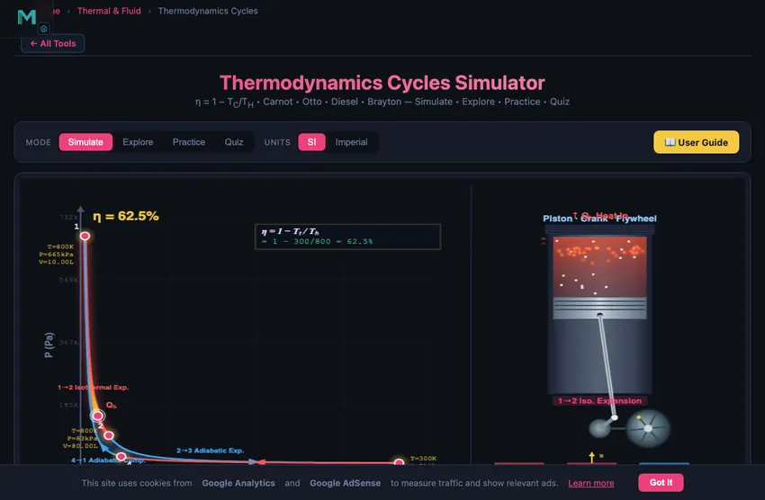
The simulator opens in Simulate mode with the Carnot cycle selected, T_hot = 800 K, T_cold = 300 K, and a compression ratio of 8. The canvas shows the PV diagram on the left with two isotherms and two adiabats forming the cycle, and an animated piston on the right. Readout cards display efficiency η, net work W_net, heat input Q_in, heat rejected Q_out, compression ratio, temperatures, and reverse COP.

Start by selecting different Cycle Types (Carnot, Otto, Diesel, Brayton) using the pill tabs. Each cycle reveals different PV diagram shapes and different controlling parameters. The Carnot cycle depends solely on temperature ratio; the Otto cycle depends on compression ratio; the Diesel cycle adds a cutoff ratio; and the Brayton cycle uses pressure ratio instead of compression ratio. Use the Presets (Ideal Carnot, Car Engine, Truck Engine, Jet Engine) to load realistic configurations quickly.

The PV diagram is the primary analysis tool. Colour-coded process lines distinguish isothermal (constant temperature), adiabatic (no heat transfer), isochoric (constant volume), and isobaric (constant pressure) processes. The enclosed area represents the net work per cycle — a larger area means more work output. Toggle Show Process Labels to see annotations on each process, and toggle Show Energy Flow to see arrows indicating heat input and heat rejection.

Key experiments to try: For the Carnot cycle, adjust T_hot and T_cold and verify that η = 1 − T_C/T_H. For the Otto cycle, increase the compression ratio from 8 to 12 and watch efficiency rise from about 56% to 63% — this is why high-compression engines are more efficient. For the Diesel cycle, increase the cutoff ratio and observe that efficiency decreases as more heat is added at constant pressure. For the Brayton cycle, increase the pressure ratio and observe the efficiency plateau predicted by the formula η = 1 − 1/r_p^(γ−1)/γ.

Switch to Explore mode to browse concept cards across three categories: Laws, Cycles, and Applications. The Laws category covers the zeroth, first, and second laws of thermodynamics, entropy as a measure of disorder, enthalpy as the heat content at constant pressure, and the Clausius inequality. The first law ΔU = Q − W is the foundation of all cycle analysis.

The Cycles category provides detailed cards on each of the four cycles, including process descriptions, efficiency formulas, PV and T-s diagram representations, and comparison tables. The Applications category covers real-world implementations: spark-ignition engines (Otto), compression-ignition engines (Diesel), gas turbines and jet engines (Brayton), geothermal and solar thermal power plants, and combined cycle systems. Each card includes formulas, worked examples, and practical engineering context.

Practice mode generates randomised thermodynamics problems. You might be asked to calculate the Carnot efficiency for given temperatures, find the net work output of an Otto cycle, determine the heat rejected in a Diesel cycle, or compute the thermal efficiency of a Brayton cycle from the pressure ratio. Enter your answer and click Check for instant feedback. Click Next Problem to generate a new scenario. Your running score tracks your improvement.

Quiz mode presents five questions per session mixing conceptual and numerical problems. Topics include identifying thermodynamic processes on PV diagrams, ranking cycles by efficiency, applying the first and second laws, calculating compression ratios, and comparing engine types. After completing the quiz, review your results and focus on any weak areas by revisiting the relevant Explore cards.

• The Carnot efficiency η = 1 − T_C/T_H sets the absolute maximum for any heat engine operating between the same temperatures. No real engine can exceed this limit — use it as a benchmark.
• On the PV diagram, the enclosed area equals the net work. A fatter cycle loop means more work per cycle. Compare the Carnot and Otto loops at the same temperature extremes to see this difference.
• For the Otto cycle, efficiency depends only on the compression ratio r and the heat capacity ratio γ = 1.4 for air. Higher r means higher efficiency, but real engines are limited by knock (detonation).
• The Diesel cycle always has lower efficiency than the Otto cycle at the same compression ratio, because constant-pressure heat addition is less efficient than constant-volume. However, Diesel engines use higher compression ratios (14–22 vs 8–12), making their actual efficiency competitive.
• Watch the energy flow arrows to visualise where heat enters and leaves the cycle. The second law requires that Q_out > 0 for any real cycle — some heat must always be rejected.
• Use this simulator alongside the Refrigeration Cycle Simulator to understand how the same thermodynamic principles operate in reverse (heat pump/refrigerator) and how COP relates to engine efficiency.