RC Circuit — Capacitor Charging & Discharging
τ = RC • V(t) = V₀(1−e−t/τ) • Charging • Discharging — Simulate • Explore • Practice • Quiz
Display Controls
Σ Live equations — values substituted from the current state
💡 What-if coach — what these numbers mean
1 Overview
The RC Circuit Simulator lets you explore how a resistor-capacitor circuit behaves during charging and discharging. The core relationship is the time constant τ = RC, which determines how quickly a capacitor charges or discharges through a resistor. During charging, the capacitor voltage follows V(t) = V₀(1 − e−t/τ), reaching 63.2% of the supply voltage after one time constant and 99.3% after five time constants (5τ).
This simulator is built for electrical engineering students, electronics technicians, and physics learners studying transient analysis, exponential decay, cutoff frequency, and RC filter design. You can adjust resistance, capacitance, and supply voltage, then watch the capacitor charge or discharge in real time with animated current flow and a live voltage-time graph.
2 Building the Circuit

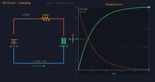
The simulator opens in Simulate mode with R = 1000 Ω, C = 100 μF, and Vsupply = 12 V, giving a time constant of τ = 100 ms. To begin:
- Throw the Charge / Discharge switch. The schematic draws a real changeover (SPDT) switch: on Charge the supply feeds R and C, and on Discharge the battery is switched out of the loop entirely and the capacitor dumps its charge through R alone.
- Drag the R slider (1 Ω–10 MΩ) and C slider (1 nF–10 mF) to change the time constant and watch the curve genuinely stretch or compress against a real time axis. Both are logarithmic — seven decades will not fit on a linear track. Type an exact value into the box beside either slider if you need one.
- Adjust the Vsupply slider (0.5–100 V) to change the voltage the capacitor charges toward.
- Pick a preset from the dropdown — standard bench, switch debounce, audio coupling, 555 timing, camera flash or a scope probe. The dropdown falls back to — Custom — as soon as you nudge anything away from a preset, and snaps back if you land on one again.
- Use the Calculations button for a full worked derivation at the cursor, and CSV / PNG to export the plotted data or the canvas.
Switch between the four modes — Simulate, Explore, Practice, Quiz — using the pill tabs at the top of the page, and between the two views — Charge / Discharge and Frequency Response — using the View tabs below them.
3 Energising the Circuit
Simulate mode is the primary interactive workspace. The canvas shows the schematic with animated current dots on the left and an oscilloscope-style graph on the right.
The graph is a real instrument, not a normalised sketch. All three axes — volts, milliamps and seconds — carry their own full scale, chosen from the standard 1-2-5 sequence and re-ranged only when the signal overflows the screen or drops below 30 % of it. A small slider move therefore visibly grows or shrinks the trace; a large one re-ranges and announces the new value on the V/div, A/div and s/div readouts above the plot.
- Transport: Pause freezes the run so you can compare two settings; the t scrubber moves the cursor anywhere in the sweep; Restart returns to t = 0. Changing R, C or V does not throw the run away — the curve moves under the cursor, which is the whole lesson.
- Speed: real RC circuits are almost never watchable — τ spans nanoseconds to minutes over this slider range. The animation is compressed and the factor is printed on the canvas (“slow motion 1 : 2700” or “fast-forward 5 : 1”), so the numbers on screen are always the real ones. The Speed dropdown scales that further.
- Display Controls (top-left of the canvas): show or hide the equation, the labels and values, the current-flow dots, the τ markers, the I(t) trace and a background grid. Your choices are remembered on your next visit.
- Right-click the canvas for copy-value, CSV and PNG export, a grid toggle and reset.
The readout cards show capacitor voltage, the time constant, instantaneous current, charge percentage, and the full energy account: energy stored in C, heat dissipated in R, and energy drawn from the supply. Watch the current start at I₀ = V/R and decay exponentially, and watch the three energy figures settle at ½CV², ½CV² and CV².
4 Circuit Theory
Explore mode organises educational content into three categories:
- Fundamentals: Covers capacitor construction, capacitance definition (C = Q/V), electric field between plates, and the relationship between charge, voltage, and energy storage.
- Time Response: Explains the exponential charging and discharging curves, the meaning of τ = RC, the 5τ rule for full charge, and how to read time-domain waveforms.
- Applications: Describes real-world uses of RC circuits including low-pass and high-pass filters (cutoff frequency fc = 1/(2πRC)), timing circuits, switch debouncing, and power supply smoothing.
Select any concept card to view a detailed explanation with formulas and an interactive canvas illustration.
5 Frequency Response — The Same R and C as a Filter
Switch the View tabs to Frequency Response and the same two components become a filter. The canvas draws a full Bode plot — magnitude in decibels above, phase below, on a six-decade logarithmic frequency axis.
- Low-pass takes the output across the capacitor: flat at 0 dB, then falling at −20 dB per decade above the cutoff, with the phase sliding from 0° to −90°.
- High-pass takes the output across the resistor: the mirror image, rising at +20 dB per decade and leading by up to +90°.
- The cutoff fc = 1/(2πRC) is marked, along with the −3 dB line and the straight-line asymptotes. At fc the reactance XC exactly equals R, the gain is 1/√2 = 0.7071, and the phase is ±45°.
- The Cursor f slider reads gain, gain in dB, phase and reactance at any frequency you like.
Like the time axis, the frequency window re-ranges only when the cutoff drifts out of the middle decades, so changing R or C visibly slides the knee along the plot instead of pinning it to the centre.
6 Try a Problem
Practice mode generates unlimited calculation problems on RC circuits. Typical questions include: “Calculate the time constant for R = 2.2 kΩ and C = 47 μF”, “What is the capacitor voltage after 3τ when charging from 0 to 12 V?”, or “Find the cutoff frequency of an RC filter with R = 1 kΩ and C = 10 μF.” Enter your numeric answer, click Check, and see a step-by-step solution.
Quiz mode draws 5 questions — a mix of multiple choice and numeric — from a pool covering the time constant, exponential decay, energy storage, the 50 % charging efficiency result and filter behaviour. The multiple-choice options are shuffled on every draw, so the answer is never in a predictable position, and every question shows why its answer is right whether you got it right or wrong.
7 Field Tips
- Remember the 5τ rule: after 5 time constants, the capacitor is at 99.3% of its final value — effectively fully charged or discharged.
- Hit Pause and then move a slider. The curve redraws under a stationary cursor, so you can read the old and new values against the same time axis instead of losing the run.
- Use the Fast preset (10 Ω, 100 μF) to see rapid charging, then switch to Slow (10 kΩ, 1000 μF) to observe a much longer time constant — and note the s/div readout changing as the scope re-ranges.
- The capacitor is half charged at t = τ ln 2 = 0.693τ, not at 0.5τ. The curve is steepest at the start, so the first half of the journey takes less than half the time.
- Charging a capacitor through a resistor is exactly 50 % efficient no matter what R you choose — watch the “Heat in R” and “From Supply” cards settle at ½CV² and CV². Making R smaller only makes the loss happen faster.
- Watch the current readout during charging — it starts at I₀ = V/R and decays to near zero, confirming exponential behaviour.
- For filter design, remember that fc = 1/(2πRC). A larger RC product gives a lower cutoff frequency.
- The energy stored in the capacitor (E = ½CV²) increases quadratically with voltage, so doubling voltage quadruples energy.
- Practice converting between time constant notation and actual seconds: τ = RC in seconds when R is in ohms and C is in farads.
Understanding RC Circuits — Free Interactive Capacitor Charging & Discharging Simulator
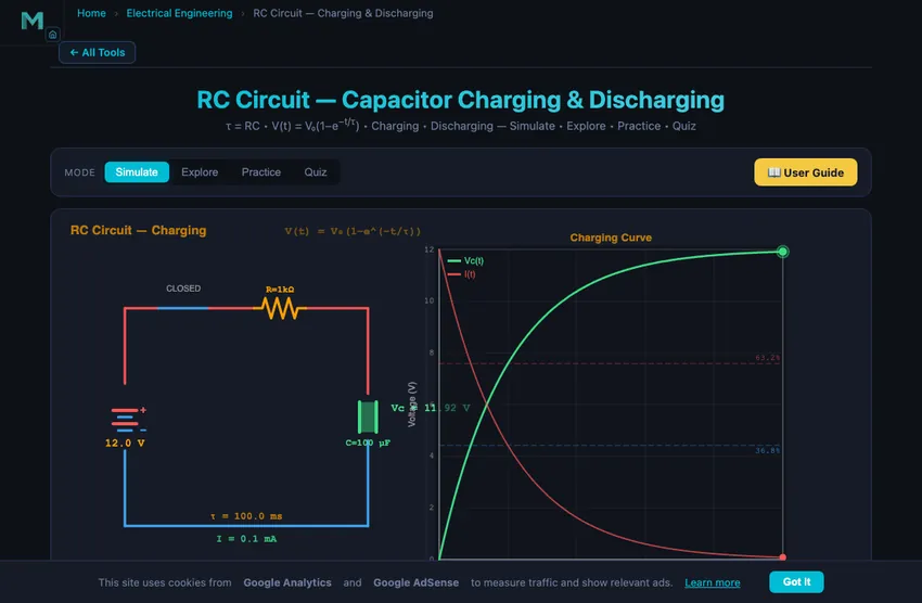
An RC circuit consists of a resistor (R) and a capacitor (C) connected in series with a voltage source. When the switch closes, the capacitor charges through the resistor following an exponential curve: V(t) = V₀(1 − e−t/τ), where τ = RC is the time constant. The time constant represents the time for the voltage to reach 63.2% of its final value. After 5τ, the capacitor is considered fully charged at 99.3% of the supply voltage. Our interactive simulator lets you set resistance from 1 Ω to 10 MΩ and capacitance from 1 nF to 10 mF, then watch the capacitor charge or discharge on a real oscilloscope-style graph with volts, milliamps and seconds per division — plus a full Bode plot of the same R and C as a low-pass or high-pass filter.
Capacitor Charging & Discharging Curves
During charging, voltage across the capacitor rises exponentially toward the supply voltage while current decreases exponentially from its initial maximum of I₀ = V/R. During discharging, the capacitor releases its stored energy: voltage decays as V(t) = V₀·e−t/τ and current flows in the opposite direction, also decaying exponentially. Note what the schematic does when you throw the switch: a discharge is not the charging circuit run backwards. The changeover switch takes the battery out of the loop altogether and leaves the capacitor to dump its charge through R alone — which is why the “from supply” energy reads zero during a discharge, and why every joule that was in the capacitor ends up as heat in the resistor.
Energy Storage and RC Filters
A capacitor stores energy as an electric field between its plates. The energy stored is given by E = ½CV². RC circuits are also fundamental building blocks for electronic filters. A low-pass RC filter passes low-frequency signals while attenuating high frequencies, with a cutoff frequency of fc = 1/(2πRC). A high-pass RC filter does the opposite, blocking DC and passing AC signals above the cutoff frequency. These filters are used extensively in audio electronics, signal processing, and power supply smoothing. The simulator’s Frequency Response view plots both, showing the −3 dB cutoff, the −20 dB-per-decade roll-off and the phase shift that goes with it — the same R and C you set for the transient, seen in the frequency domain.
Practical Applications of RC Circuits
RC circuits appear everywhere in electronics: timing circuits in 555 timers, debouncing switches, smoothing rectified power supplies, coupling and decoupling signals between amplifier stages, and setting the bandwidth of communication receivers. The time constant τ = RC is the key design parameter — choosing the right combination of R and C determines how fast the circuit responds. Engineers use RC calculations daily when designing filters, timing delays, and transient response networks.
The Five-Tau Rule — The Single Most Useful Number in RC Analysis
Every electronics class learns it, but here is the rule in the form that survives long after exam questions are forgotten: after five time constants, an RC circuit is settled to better than 1% accuracy. The maths:
| Time | Voltage as % of final | Remaining error |
|---|---|---|
| 0 τ (immediately after switch close) | 0 % | 100 % (full final voltage to go) |
| 1 τ | 63.2 % | 36.8 % |
| 2 τ | 86.5 % | 13.5 % |
| 3 τ | 95.0 % | 5.0 % |
| 4 τ | 98.2 % | 1.8 % |
| 5 τ | 99.3 % | 0.7 % |
| 7 τ | 99.91 % | 0.09 % |
The 63.2 % at one τ is the formal definition: 1 − 1/e ≈ 0.632. It is the answer that distinguishes a candidate who memorised the formula from one who can derive it. The 99.3 % at five τ is the answer that distinguishes a working engineer from one who’s still in school. After 5τ most digital designs are settled enough that you can clock the next operation.
A Real RC Worked Example — A 1 ms Debounce
Push-button switches don’t close cleanly. They “bounce” for the first 1−10 ms after contact — mechanical chatter that produces a noisy signal. The simplest debounce uses an RC low-pass filter: pick τ that absorbs the bounce while still being fast enough not to be felt as input lag. Try 1 ms.
Need τ = RC = 1 ms. Common solution: R = 10 kΩ, C = 100 nF. Verify: τ = 10,000 × 100×10−9 = 10−3 s = 1 ms ✓.
Load the Switch debounce preset and you get exactly that circuit. In the charge/discharge view the output needs about 5τ = 5 ms to settle to a clean level — well inside the latency a finger can feel. Switch to the Frequency Response view and the same pair reads fc = 1/(2π × 10 kΩ × 100 nF) = 159 Hz, so the kilohertz-rate chatter of the bouncing contact lands far out on the −20 dB/decade slope and is heavily attenuated. Those are two views of one design decision. This trick appears in every keyboard, remote control, and microcontroller input designed since the 1970s.
Energy in the Capacitor — Where Did Half of It Go?
A subtle puzzle. When you charge a capacitor C from 0 to V0 through a resistor R, the energy supplied by the battery is Q×V0 = C·V0². The energy stored in the capacitor is ½C·V0². Where did the other half go?
Answer: dissipated in the resistor as heat, exactly ½C·V0². And here’s the strange part — this is true regardless of how big the resistor is. A 1 Ω resistor and a 1 MΩ resistor both dissipate the same total energy charging the same capacitor. The 1 MΩ case just takes much longer to do it. This 50 % charging efficiency is a fundamental limit of RC charging and is why switch-mode power supplies (which use inductors to achieve near-100 % efficiency) replaced linear RC supplies for any significant power transfer.
References for RC Analysis
- Sedra, A. S. & Smith, K. C. — Microelectronic Circuits, 8th ed., Chapter 1.
- Horowitz & Hill — The Art of Electronics, 3rd ed. The practical bench reference.
- Forrest Mims — Engineer’s Mini-Notebook: 555 Timer IC Circuits. Forty pages, every variant of RC timing you’ll need.
Explore Related Simulators
If you found this RC Circuit simulator helpful, explore our Ohm’s Law simulator, RLC Circuit simulator, Transformer simulator, and Wheatstone Bridge simulator, and Resistor Color Code Calculator for more hands-on practice with electrical circuits.
Updated