Transformer — Step-Up & Step-Down
Turns Ratio • E = 4.44 f N Φₘ • Equivalent Circuit • Regulation & Efficiency • OC / SC Tests — Simulate • Tests • Explore • Practice • Quiz
Display Controls
some texts use N₁/N₂
Σ Live equations — values substituted from current state
💡 What-if coach — insights from current values
1 Overview
The Transformer Simulator is built around a nameplate, not a turns ratio. You set the rating, the primary voltage, the frequency and the turns; from those the simulator derives the core cross-section, the winding resistance and leakage reactance, and the magnetising branch — the whole equivalent circuit — and then solves it exactly. Change any slider and the machine changes with it.
That means you can explore step-up and step-down transformation and the turns ratio (a = N₂/N₁), but also the things a turns ratio alone cannot show: the EMF equation E = 4.44 f N Φₘ setting the core flux density, core saturation when the volts-per-turn-per-hertz is wrong, voltage regulation at any power factor including the leading loads that make it negative, and the load at which efficiency peaks because copper loss has grown to equal iron loss.
A separate Tests tab runs the two classical bench tests — open-circuit and short-circuit — on whichever machine you have set up, and shows how their meter readings recover the equivalent circuit you started from.
This tool is designed for electrical engineering students, power systems trainees, and physics learners studying Faraday’s law, voltage transformation, transformer testing, and real-world losses.
2 Building the Circuit
The canvas is at the top, and the control panel sits directly beneath it. The panel’s own top line is a ribbon holding everything that changes what machine this is and everything you can do to it: the Preset dropdown, the Real transformer and Leading load toggles, then Calculations and icon buttons for undo, redo, reset, CSV and PNG (hover any of them for its name). Below the panel sit the readout cards.
The simulator opens in Simulate mode with a 1.6 kVA machine: V₁ = 120 V, N₁ = 100 turns, N₂ = 200 turns, 50 Hz, feeding a 60 Ω resistor, ideal (lossless). That gives a turns ratio of 2.0, a 240 V step-up output, and a core flux density of 1.17 T — a sensible working point for silicon steel.
Nameplate & supply.
- N₁ and N₂ — 5 to 50,000 turns, and the first thing to reach for. If N₂ > N₁ the transformer steps up; if N₂ < N₁ it steps down. N₁ also sets the flux: fewer turns means more flux in the same iron.
- V₁ Primary (V) — 6 V to 132 kV. The slider steps through standard system voltages (110, 230, 415, 11 k, 33 k, 132 k…); type any value in the box.
- S Rating (kVA) — 0.05 kVA to 5,000 kVA. The slider walks the standard IEC ratings; the box beside it accepts anything in between. The rating decides the core cross-section and, through published per-unit design data, the winding resistance, the leakage reactance, the no-load current and the core loss.
- f Frequency (Hz) — 16 to 400 Hz, with 50 / 60 / 400 Hz shortcut chips beside the section heading. Frequency appears in the EMF equation, so it changes the core flux directly.
Load. The dropdown beside the Load heading offers two ways of asking for the same thing:
- A resistor across the secondary — a real resistor, so the power factor is 1. Good for the basic voltage-and-current story and for impedance matching.
- A current, as % of rated, at a power factor — a load current expressed as a percentage of rated secondary current, at a power factor you choose between 0.30 and 1.00. This is how every textbook problem is posed, and it is the only way to reach the regulation and power-factor lessons. The Leading load chip in the ribbon makes it capacitive; it stays greyed out while the load is a plain resistor, because a resistor has no power factor to lead or lag.
Every slider carries a live value with its unit, and a − / box / + stepper. On the rating, voltage, turns and load-resistance sliders the stepper walks the standard sizes — one press moves 11 kV to 22 kV rather than nudging it by a volt — while the box still accepts any value in between.
Tick Real transformer in the ribbon to switch from the ideal machine to the real one: winding drops, magnetising current, copper and iron losses, and a secondary voltage that sags under load. It is a lens over whatever machine you have loaded rather than a different machine, so it starts off — including on every preset — and the preset dropdown goes on naming the transformer once you switch it on.
Navigate through Simulate, Tests, Explore, Practice, and Quiz modes using the pill tabs at the top.
3 Energising the Circuit
The View bar above the canvas switches between four ways of looking at the same solved machine:
- Machine — the physical picture. Two windings on a laminated core, flux animating through the iron at a clearly-labelled slow motion, an oscilloscope panel showing both voltage waveforms at a real volts-per-division scale, and (in real mode) a loss breakdown. The core caption shows the flux density Bₘ and turns red when the iron saturates.
- Equivalent Circuit — the exact T-model referred to the primary, with R₁, X₁, R₂′, X₂′, R₀ and Xₘ carrying the values your nameplate produces, plus the approximate circuit and %R, %X, %Z below it.
- Phasor Diagram — V₁, V₂′, I₁ and I₀ drawn to scale from the solved complex quantities, with the primary power-factor angle marked. The gap between the two voltage tips is the regulation.
- Efficiency Curve — efficiency and regulation swept across 0–125% load, with the copper and iron loss curves underneath. The peak is marked, and a second marker shows where your current operating point sits on it.
The readout cards show turns ratio, type, secondary voltage, both currents, the load as a percentage of rated, input and output power, efficiency, and — in real mode — voltage regulation, core flux density Bₘ, no-load current I₀, and the primary power factor. Cards that mean nothing in ideal mode are hidden rather than filled with a dash.
4 Circuit Theory
Explore mode organises transformer theory into three categories:
- Transformer Basics: Covers electromagnetic induction, Faraday’s law, turns ratio, ideal transformer equations (V₂/V₁ = N₂/N₁), and the principle that power is conserved in an ideal transformer.
- Losses & Efficiency: Explains copper losses (I²R heating in windings), iron losses (hysteresis loss from magnetic domain reversal and eddy current loss from circulating currents in the core), and how laminated silicon steel cores minimise eddy currents.
- Testing & Performance: The equivalent circuit and what each element represents, the open-circuit and short-circuit tests, voltage regulation including the leading-load case where it goes negative, and percentage impedance and the fault current it implies.
- Applications: Describes power transmission (step-up for long-distance, step-down for distribution), isolation transformers, instrument transformers (CTs and PTs), and autotransformers.
Each concept card provides formulas, explanations, and an interactive canvas illustration.
5 The Tests Tab — OC, SC and Load Test
Nobody load-tests a 100 MVA transformer — you would need a 100 MVA load and would waste 100 MVA of energy doing it. Instead two small tests, together consuming about 1% of the rating, determine the whole equivalent circuit. The Tests tab runs both on whichever machine you set up in Simulate mode, so changing the nameplate there moves every reading here.
- Open-Circuit (no-load) test. Rated voltage on the LV winding, the HV winding open. Only the no-load current flows, so the I²R term is negligible and the wattmeter reads core loss. From V₀, I₀ and W₀ the panel derives cos φ₀, Iw, Iμ, and then R₀ and Xₘ.
- Short-Circuit (impedance) test. The LV winding is bolted shut and the HV winding is fed from a supply raised until rated current flows — only a few percent of rated voltage, and that percentage is %Z. The core is barely magnetised, so the wattmeter reads full-load copper loss. From Vsc, Isc and Wsc the panel derives Zeq, Req and Xeq.
- Load test — η & regulation. The direct test: efficiency and regulation measured point by point across the load range, with a table at the classical 25 / 50 / 75 / 100 / 125% points, the maximum-efficiency load worked out, and a demonstration that the same answer comes out of the OC and SC results alone.
Each test ends with a “does the test recover the machine?” table comparing the derived parameters against the ones the model actually holds. They agree to within a fraction of a percent — and the small residual is real, not rounding: the OC wattmeter also sees the I₀²R loss in its own winding, and the SC test ignores the magnetising branch. Those are exactly the approximations the standard method makes on a real bench.
Both CSV and PNG exports are available for whichever test is on screen.
6 Try a Problem
Practice mode generates problems such as: “A transformer has N₁ = 200 turns and N₂ = 50 turns. If V₁ = 240 V, find V₂”, “Calculate primary current if secondary current is 2 A and turns ratio a = N₂/N₁ = 5”, or “Find efficiency if Pin = 500 W and total losses are 25 W.” Enter your answer and receive a step-by-step solution.
Quiz mode presents 5 multiple-choice questions covering turns ratio, step-up vs step-down identification, current transformation, copper and iron losses, and efficiency calculations. Review your score and detailed explanations at the end.
7 Tools, Export & Shortcuts
- Type exact values: every slider has a companion number box — type a precise V₁, N₁, N₂, or RL instead of dragging.
- Preset dropdown: six machines that exist. Bench 1.6 kVA (the opening state), Doorbell 240/12 V (a 100 VA control transformer, and its 8.7% regulation is why they sag), 1:1 Isolation 2.5 kVA, Distribution 1 MVA (11 kV/415 V at 0.8 lagging, the case every power-systems course works through), Generator step-up 5 MVA (11 kV to a 132 kV line), and Under-turned core — the same bench machine with half the primary turns, so the iron is driven to 4.7 T and the core caption turns red before you have touched anything else.
Every preset arrives as an ideal transformer, so you meet the machine as a clean turns-ratio problem first. Tick Real transformer to lay the winding drops, the magnetising current and the losses over the top of it — on the under-turned core that is when the magnetising current bolts to tens of amps and the efficiency collapses. The dropdown keeps naming the machine while you switch that lens on and off; only moving a slider makes it read — Custom —. - Calculations: the first button in the ribbon opens the step-by-step derivation for whatever the machine is doing right now — core area, EMF equation, machine parameters, the circuit solve, regulation, losses, efficiency, and a power-balance check.
- View bar: Machine, Equivalent Circuit, Phasor Diagram and Efficiency Curve.
- Display Controls (the chip on the canvas): six switches over what the canvas draws.
- Equation on canvas — the classical turns-ratio equation across the top of the machine view.
- Labels & values — every value annotated on the drawing itself: turns, voltages, currents, the load, the nameplate line and the core flux density. Turning it off leaves a clean schematic worth printing or projecting. The core still turns red when it saturates, because that is a warning rather than a label.
- Waveform scope — the oscilloscope panel under the machine.
- Loss breakdown — the copper/iron loss box on the machine view, and the two dashed loss curves on the Efficiency Curve view.
- Animate flux & current — freezes the flux arrows and the current dots where they are. The sliders still move everything else, so this is how you take a screenshot, or make a slow device comfortable.
- Background grid — a reference grid behind every view.
- Live equations & What-if coach: collapsible panels below the controls show the substituted formulas and plain-language insights about your current settings.
- Show Equation / Show Grid: toggle the on-canvas turns-ratio equation and a background reference grid.
- Export: CSV sweeps the load from no load to 125% and records V₂, I₂, input and output power, copper and iron loss, efficiency and regulation at each point, with the machine's full parameter set in the header comments; PNG saves the canvas as a watermarked image. Both are also on the canvas right-click menu, and the Tests tab has its own pair.
- Keyboard: Ctrl+Z undo, Ctrl+Shift+Z redo, Esc closes the calculation modal.
8 Field Tips
- Every preset lands ideal on purpose. Read the turns-ratio story first — a, V₂, the two currents, power in equals power out — then tick Real transformer and watch what it costs: V₂ sags, I₀ appears, and the efficiency card drops off 100%.
- Set N₁ = N₂ to create a 1:1 isolation transformer — voltage stays the same but the circuits are galvanically isolated.
- Notice that when you step up voltage, current steps down proportionally — power is conserved (P = V × I).
- With the Real Transformer mode on, try increasing load current by lowering RL. Watch copper losses (I²R) increase significantly while iron losses remain roughly constant.
- For maximum efficiency, transformers operate best at or near rated load. Very light loads give poor efficiency because iron losses dominate.
- Remember: turns ratio a = N₂/N₁. If a > 1, it steps up voltage; if a < 1, it steps down voltage.
- Halve N₁ and watch Bₘ double. The EMF equation Φₘ = V/(4.44 f N) is the whole reason a transformer has the number of turns it does — and past about 1.7 T the core saturates and the magnetising current runs away.
- Switch the frequency from 50 to 60 Hz at fixed voltage and the flux falls by a factor of 60/50. Now do it the other way: a 60 Hz transformer on a 50 Hz supply is over-fluxed by 20% and can overheat with nothing connected to it.
- In % of rated + PF mode, set the power factor to 0.8 and flip between lagging and leading. On the 1 MVA distribution preset the leading case gives negative regulation — the secondary voltage rises under load, because %X·sinφ has overtaken %R·cosφ.
- Open the Efficiency Curve view and find where the copper and iron loss curves cross. That crossing is the efficiency peak, and it is why distribution transformers are sized to run at 50–75% of rating rather than flat out.
- Run the Short-Circuit test and read %Z. A dead short at full voltage draws roughly 100/%Z times rated current — the number that sizes the switchgear.
- Use Practice mode to drill the equations: V₂ = a×V₁, E = 4.44 f N Φₘ, Reg% ≈ %R·cosφ ± %X·sinφ, and η = Pout/Pin × 100%.
Understanding Transformers — Free Interactive Step-Up & Step-Down Simulator
A transformer changes AC voltage using two coils on a shared iron core. The turns ratio a = N₂/N₁ sets the output: V₂ = a × V₁. When a > 1 it steps voltage up and current down; when a < 1 it steps down. An ideal transformer conserves power. A real one loses 1–5% to copper and iron, and its secondary voltage sags under load — that drop is called voltage regulation.
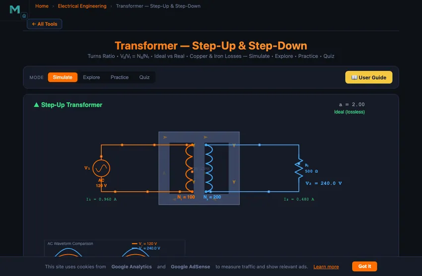
A transformer is an electrical device that transfers energy between circuits through electromagnetic induction. It consists of two or more coils (windings) wrapped around a common magnetic core. The primary winding receives AC voltage, creating a changing magnetic flux in the core, which induces a voltage in the secondary winding according to Faraday’s law of electromagnetic induction. The voltage ratio between the windings is determined by the turns ratio: V₂/V₁ = N₂/N₁. Our interactive simulator lets you adjust primary voltage, winding turns, and load resistance while watching animated magnetic flux flow through the core and comparing AC waveforms in real time.
Step-Up vs Step-Down Transformers
A step-up transformer has more turns on the secondary winding than the primary (N₂ > N₁), which increases the output voltage while proportionally decreasing the output current. This type is used in power transmission to raise voltage for long-distance delivery, reducing I²R losses in the cables. A step-down transformer has fewer secondary turns (N₂ < N₁), lowering the voltage for safe distribution to homes and equipment. In an ideal transformer, power is fully conserved: P₁ = V₁ × I₁ = V₂ × I₂ = P₂.
The EMF Equation — What Actually Decides the Flux
The turns ratio tells you the voltage, but it does not tell you how much iron the transformer needs, why it hums, or why it can burn out with nothing plugged into it. The equation that does is the EMF equation:
E = 4.44 × f × N × Φm = 4.44 × f × N × Bm × A
The 4.44 is 2π/√2 — the factor that turns a peak rate of change of flux into an RMS voltage. Read forwards it gives the induced EMF. Read backwards it gives something far more useful:
Φm = V / (4.44 × f × N)
The flux in the core is fixed by the applied voltage, the frequency and the turns. The load appears nowhere in it. Three consequences follow immediately, and all three are things students are usually asked to memorise instead of derive:
- Iron loss is constant at all loads. Core loss depends on the flux, and the flux does not change when you connect a load. That is why a transformer left energised overnight costs money for nothing, and why efficiency is poor at light load.
- Too few turns saturates the core. Halve N₁ and you double Bm. Silicon steel bends over at about 1.7 T and is finished by 2.0 T; past the knee the magnetising current rises far faster than the voltage, and the winding cooks. In the simulator the Under-turned core preset does exactly this — the core caption turns red and the no-load current jumps from under an amp to tens of amps.
- Frequency matters as much as voltage. Since Φ ∝ V/f, a 60 Hz transformer connected to a 50 Hz supply of the same voltage is over-fluxed by 20%. This is a real and common failure: the machine overheats at no load. The reverse — a 50 Hz design on 60 Hz — is harmless, just under-worked iron.
A designer works this in the other direction. The rating buys a core of a certain cross-section (roughly Acm² ≈ 1.15√VA for a small transformer), a working flux density of 1.1–1.5 T is chosen, and the turns follow. Move any slider in the simulator and you can watch Bm respond.
Transformer Losses and Efficiency
Real transformers experience two categories of energy loss. Copper losses (I²R losses) occur because winding wire has finite resistance, generating heat proportional to the square of the current. Iron losses (core losses) include hysteresis loss — energy wasted as magnetic domains in the core reverse direction each AC cycle — and eddy current loss, caused by circulating currents induced in the core material. To minimise eddy currents, transformer cores are made from thin laminated sheets of silicon steel. Well-designed power transformers achieve efficiencies of 95% to 99%, making them among the most efficient electrical machines.
Open-Circuit and Short-Circuit Tests — Finding the Equivalent Circuit
A real transformer is an ideal one wrapped in four imperfections: winding resistance (R₁, R₂), leakage reactance (X₁, X₂) from flux that links one winding but not the other, a core-loss resistance R₀, and a magnetising reactance Xm. Together they form the equivalent circuit, and every number a power engineer needs comes out of it.
You cannot measure those elements directly. You can measure them with two small tests that, between them, consume about 1% of the transformer’s rating:
| Open-circuit (no-load) test | Short-circuit (impedance) test | |
|---|---|---|
| Fed from | LV winding, HV winding open | HV winding, LV winding shorted |
| Applied voltage | Rated | 4–6% of rated, raised until rated current flows |
| Why that way | Only I₀ flows, so I²R is negligible | Flux is tiny, so core loss is negligible |
| Wattmeter reads | Core loss Pfe | Full-load copper loss Pcu |
| Gives | cos φ₀ = W₀/(V₀I₀), then R₀ = V₀/Iw and Xm = V₀/Iμ | Zeq = Vsc/Isc, Req = Wsc/Isc², Xeq = √(Zeq² − Req²) |
The short-circuit voltage, as a percentage of rated, is the percentage impedance %Z stamped on every nameplate. It is not a curiosity: a bolted fault on the secondary at full voltage draws roughly 100/%Z times rated current, so a 5% transformer delivers about 20 times rated current into a short. That number sizes the circuit breakers. It also decides how two transformers share load when paralleled — they divide it in inverse proportion to their impedances, which is why paralleling a 4% and a 6% unit overloads the 4% one.
With Pfe from one test and Pcu from the other, the efficiency at any load follows without ever connecting a load: η = xS·cosφ / (xS·cosφ + x²Pcu,FL + Pfe). The simulator’s Tests tab runs both tests on whatever machine you have set up and shows the derived parameters beside the ones the model actually holds — they agree to a fraction of a percent, and the residual is the approximation each test genuinely makes.
Voltage Regulation — and When It Goes Negative
Load a transformer and its secondary voltage drops, because the current has to flow through Req and Xeq. Voltage regulation expresses that as a percentage:
Reg% = (V₂ at no load − V₂ at load) / V₂ at load × 100
The working approximation, accurate to a few tenths of a percent on any real machine, is Reg% ≈ %R·cosφ + %X·sinφ for a lagging load. Its power-factor dependence is the whole lesson: an inductive load makes regulation worse because the reactive drop adds, which is one of the reasons power factor correction is worth paying for.
For a leading (capacitive) load the reactive term subtracts. And if %X·sinφ exceeds %R·cosφ, regulation goes negative — the secondary voltage rises under load. That is not a textbook curiosity; it is why long, lightly-loaded cable networks and over-corrected installations can see overvoltage. Large transformers, where %X dominates %R, do it readily; small ones, where the resistance dominates, do not. Load the 1 MVA distribution preset at 0.8 leading and watch the number go below zero.
Transformer Equations & Calculations
The fundamental transformer equations are: Turns ratio a = N₂/N₁, V₂ = a × V₁, and I₂ = I₁/a (ideal). Efficiency is calculated as η = (P₂/P₁) × 100%. Voltage regulation measures the drop from no-load to full-load secondary voltage: VR% = (V₂₀ₗ − V₂ₗₗ)/V₂ₗₗ × 100%. These formulas are essential for transformer design and selection in power systems engineering.
From 11 kV to 415 V — A Real Distribution Transformer in One Calculation
The transformer that feeds your neighbourhood typically steps 11 kV three-phase down to 415 V three-phase (240 V per phase to neutral). It is a 500 kVA unit, often a Delta-Star configuration, mounted on a pole or in a kiosk. Walk through the calculation:
| Step | Working | Result |
|---|---|---|
| Turns ratio (phase to phase) | a = Ns/Np = Vs/Vp = 415/11000 (the reciprocal, 26.5 : 1, is the primary-to-secondary ratio some textbooks call the turns ratio) | 0.0377 (step-down) |
| Primary current at rated load | Ip = S/(√3·Vp) = 500000/(√3·11000) | 26.2 A |
| Secondary current at rated load | Is = S/(√3·Vs) = 500000/(√3·415) | 695 A |
| Current ratio (cross-check) | Ip/Is = 26.2/695 (I1 = a·I2) | 0.0377 ✓ (matches a) |
695 A at 415 V is what the cables coming out of the bottom of the transformer have to carry. That is why the low-voltage cables are so much thicker than the high-voltage ones above. Energy is conserved at the transformer, but it gets repackaged from low-current high-voltage into high-current low-voltage. Each form has its own engineering trade-offs — insulation cost on the HV side, conductor cost on the LV side.
Why You Cannot Use a Transformer on DC
This question comes up in every first-year electrical class. The textbook answer is “because transformers need a changing flux to induce EMF.” That is true but unsatisfying. Here is what actually happens if you connect a DC supply to a transformer primary:
- At the instant you close the switch, the current rises rapidly from zero. The changing current creates changing flux. The secondary sees an induced EMF — briefly. This is the transient.
- Once the current reaches steady-state DC value, the flux is also steady. dφ/dt = 0, so the secondary EMF is zero. The induced voltage you wanted has vanished.
- Meanwhile, the primary current is now limited only by the winding resistance (a few ohms at most), so a typical 230 V supply produces tens of amperes through the primary. The winding overheats in seconds and melts.
DC into a transformer is not just “useless” — it destroys the transformer. The lab demonstration is usually done with a heavily current-limited supply or with a fast circuit breaker.
Where Real Transformers Lose Efficiency
A modern distribution transformer is 97−99% efficient. The losing 1−3% comes from two distinct sources, each behaving differently with load:
- Copper losses (I²R). Heat in the winding wire, proportional to load squared. At no load these are zero; at full load they reach maximum. Designers oversize wire gauge to push these down.
- Iron losses (hysteresis + eddy currents). Heat in the core, roughly constant regardless of load. Hysteresis is the energy needed to magnetise and demagnetise the silicon steel each cycle. Eddy currents are local circulating currents in the core; thin laminations and silicon doping reduce them. These are the losses you pay 24/7 even if no load is drawing power.
That trade-off is why every distribution transformer has a “maximum efficiency point” somewhere around 50–70 % of rated load — the point where copper losses equal iron losses. The efficiency curve dips slightly at full load and more sharply at very light loads.
Standards and References for Transformer Design
- Chapman, S. J. — Electric Machinery Fundamentals, 5th ed., Chapter 2 (Transformers). The standard undergraduate reference.
- IEEE Std C57.12.00 — Standard for General Requirements for Liquid-Immersed Distribution, Power, and Regulating Transformers.
- IEC 60076 (multi-part) — the international transformer standard, covering rating, losses, and dielectric performance.
- Kothari, D. P. & Nagrath, I. J. — Electric Machines, 5th ed., for worked examples on three-phase transformer calculations.
Explore Related Simulators
If you found this Transformer simulator helpful, explore our Ohm’s Law simulator, RC Circuit simulator, Induction Motor simulator, RLC Circuit simulator, Wheatstone Bridge simulator, Star-Delta Conversion simulator, and Faraday's Law simulator, the House Wiring Simulator, and the Magnetic Playground (the field of a solenoid and electromagnetic induction) for more hands-on practice.
Updated