How does an AC generator work?

An AC generator works on Faraday's law of electromagnetic induction. A rectangular coil rotates inside a magnetic field, and the changing magnetic flux through the coil induces an alternating EMF. The EMF follows a sinusoidal pattern: e(t) = NBAw sin(wt), where N is the number of turns, B is magnetic flux density, A is coil area, and w is angular velocity.

What is the EMF equation of an alternator?

The peak EMF of an alternator is E0 = NBAw, where N = number of turns, B = magnetic flux density in Tesla, A = coil area in m2, and w = angular velocity in rad/s. The RMS EMF is E_rms = E0 / sqrt(2) = 0.707 x E0. The instantaneous EMF varies sinusoidally as e(t) = E0 x sin(wt).

What is the difference between AC and DC generators?

An AC generator uses slip rings to maintain continuous contact with the rotating coil, producing alternating current that reverses direction each half cycle. A DC generator uses a commutator (split rings) that reverses connections every half turn, converting the alternating EMF into unidirectional (pulsating DC) output. AC generators are simpler, more reliable, and used for power generation, while DC generators are used for battery charging and electroplating.

AC Generator Simulator

EMF • Waveform • RMS Voltage • Frequency • Power — Simulate • Explore • Practice • Quiz

Mode

📖 User Guide

Turns N 100

Flux B (T) 0.50 T

Area A (m²) 0.010 m²

Speed (RPM) 1500 RPM

Load R (Ω) 100 Ω

Peak EMF

0 V

RMS EMF

0 V

Frequency

0 Hz

RMS Current

0 A

Power

0 W

Period

0 ms

User Guide — AC Generator Simulator

1 Overview

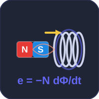
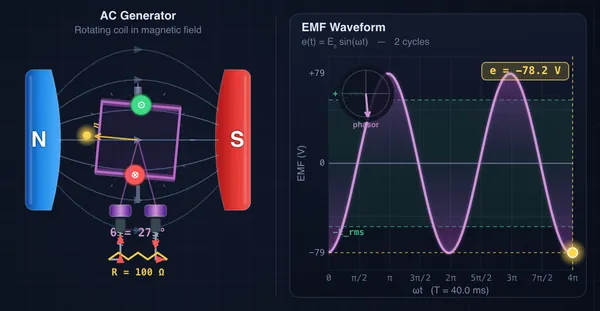
The AC Generator Simulator demonstrates how a rotating coil inside a magnetic field generates a sinusoidal electromotive force (EMF) through electromagnetic induction. Based on Faraday’s law, the instantaneous EMF is e(t) = NBAω sin(ωt), where N is the number of turns, B is the magnetic flux density in Tesla, A is the coil area in m², and ω is the angular velocity in rad/s. You can adjust each parameter and observe the rotating coil animation alongside the real-time sinusoidal waveform, peak voltage, RMS value, frequency, and power output.

This tool is built for electrical engineering students studying electromagnetic induction, engineering trainees learning alternator principles, and physics learners exploring the relationship between mechanical rotation and AC power generation.

2 Getting Started

The simulator opens in Simulate mode with N = 100 turns, B = 0.50 T, A = 0.010 m², speed = 1500 RPM, and R_load = 100 Ω. To begin:

Drag the Turns N slider (1–500) to change the number of coil turns. More turns means higher peak EMF.
Adjust the Flux B slider (0.1–2.0 T) to change the magnetic field strength.
Change the Area A slider (0.001–0.1 m²) to modify the coil cross-sectional area.
Drag the Speed slider (100–3600 RPM) to control rotational speed. This changes both peak EMF and frequency simultaneously.
Set the Load R slider (1–1000 Ω) to add a resistive load and see current and power output.
Click Play to start the coil rotation animation.

3 Simulate Mode

Simulate mode is the main interactive workspace. The canvas shows a rotating rectangular coil inside magnetic poles and a live sinusoidal EMF waveform graph. Key controls and relationships:

Turns N: Peak EMF is directly proportional to N. Doubling turns doubles E₀.
Flux B (Tesla): Peak EMF is directly proportional to B. Stronger magnets produce higher voltage.
Area A (m²): Peak EMF scales linearly with coil area. Larger coil area captures more magnetic flux.
Speed (RPM): Determines both peak EMF and frequency. For a 2-pole generator, f = RPM/60. At 3000 RPM, f = 50 Hz; at 3600 RPM, f = 60 Hz.
Load R (Ω): With a load connected, I_rms = E_rms/R and power P = E_rms²/R.
Play button: Starts/stops the coil rotation animation synchronised with the waveform.

Readout cards display: peak EMF (E₀ = NBAω), RMS EMF (E₀/√2), frequency (Hz), RMS current (A), power (W), and period (ms).

4 Explore Mode

Explore mode organises generator theory into three categories:

Fundamentals: Covers Faraday’s law of electromagnetic induction, magnetic flux linkage (Φ = NBA cos(ωt)), the relationship between flux change and induced EMF (e = −dΦ/dt), and how sinusoidal waveforms arise from uniform circular motion.
Components: Describes the stator (permanent magnets or field windings providing the magnetic field), rotor (rotating coil/armature), slip rings (continuous rings for AC output), and brushes (carbon contacts). Explains the difference between AC generators (slip rings) and DC generators (split-ring commutator).
Applications: Covers power station synchronous generators, automotive alternators, wind turbine generators, the multi-pole frequency formula f = (P × n)/120, and three-phase generation with 120° phase displacement.

5 Practice & Quiz

Practice mode generates problems such as: “A coil with 200 turns and area 0.05 m² rotates at 3000 RPM in a 0.8 T field. Calculate the peak EMF”, “Find the RMS voltage if E₀ = 340 V”, or “What speed in RPM is needed to generate 50 Hz with a 4-pole alternator?” Enter your answer and receive step-by-step solutions.

Quiz mode presents 5 multiple-choice questions covering the EMF equation, Faraday’s law, RMS vs peak relationships, frequency calculation, and generator component identification. Review your score and detailed explanations at the end.

6 Tips & Best Practices

The peak EMF equation E₀ = NBAω contains four independent variables. Change one at a time to see its individual effect on the waveform.
Set speed to 3000 RPM for a 50 Hz output or 3600 RPM for 60 Hz — these are the standard power generation frequencies worldwide.
The RMS value is always E₀/√2 ≈ 0.707 × E₀. RMS is the value quoted for mains voltage (e.g., 230 V RMS in Europe corresponds to 325 V peak).
Notice that increasing speed raises both voltage and frequency simultaneously. In real power plants, frequency must be precisely controlled by governing the prime mover speed.
Watch the rotating coil animation: EMF is maximum when the coil is parallel to the field (maximum rate of flux change) and zero when perpendicular (momentarily no flux change).
For multi-pole generators, use f = (P × n)/120. A 4-pole alternator only needs 1500 RPM for 50 Hz, halving the required speed.
Practise converting between RPM, angular velocity (ω = 2πn/60), frequency, and period to build fluency with AC generation calculations.

Understanding AC Generators — Free Interactive Simulator

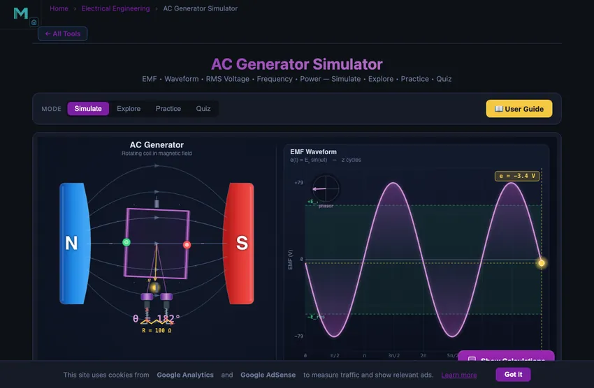
An AC generator (alternator) is a machine that converts mechanical rotational energy into alternating current electrical energy through electromagnetic induction. Based on Faraday’s law, when a coil rotates inside a magnetic field, the continuously changing magnetic flux linkage induces an electromotive force (EMF) that alternates sinusoidally. The fundamental equation governing the instantaneous EMF is e(t) = NBAω sin(ωt), where N is the number of turns in the coil, B is the magnetic flux density, A is the coil area, and ω is the angular velocity in radians per second. Our interactive simulator lets you adjust each of these parameters and observe how they affect the generated waveform, peak voltage, RMS voltage, frequency, and power output in real time.

EMF Equation and Sinusoidal Waveform

The peak EMF (E₀) of an AC generator is given by E₀ = NBAω. Since the coil rotates at a constant angular velocity, the instantaneous EMF traces a perfect sine wave. The RMS (root mean square) voltage is E₀ / √2 ≈ 0.707 × E₀, which represents the equivalent DC voltage that would deliver the same power to a resistive load. For a two-pole generator rotating at n RPM, the frequency is f = n / 60 Hz, and the period is T = 1/f seconds. Increasing the rotational speed raises both the frequency and the peak EMF, while increasing the number of turns, flux density, or coil area increases only the peak EMF without changing the frequency.

Components of an AC Generator

A basic AC generator consists of a stator (stationary part providing the magnetic field using permanent magnets or field windings), a rotor (rotating coil or armature), slip rings (continuous metal rings attached to the rotor shaft that maintain electrical contact with external circuits), and brushes (carbon or graphite contacts that press against the slip rings). Unlike a DC generator which uses a split-ring commutator, the AC generator’s slip rings allow the alternating EMF to pass through unchanged, producing a pure sinusoidal output.

Applications of AC Generators

AC generators are the backbone of modern electrical power systems. Large synchronous generators in power plants produce three-phase AC power at 50 Hz or 60 Hz for the electrical grid. Smaller alternators are used in automobiles, portable generators, and wind turbines. The frequency of the generated voltage is determined by the rotational speed and the number of magnetic poles: f = (P × n) / 120, where P is the number of poles. Three-phase generators produce three sinusoidal voltages displaced by 120°, enabling efficient power transmission over long distances.

Who Uses This Simulator?

This AC generator simulator is designed for electrical engineering students studying electromagnetic induction and AC machines, technical trainees learning about power generation fundamentals, industrial technicians understanding alternator behaviour, and instructors teaching Faraday’s law and AC circuit theory. It provides hands-on understanding of generator operation without requiring physical laboratory equipment.

Explore Related Simulators

If you found this AC Generator simulator helpful, explore our DC Motor Simulator, Transformer Simulator, RLC Circuit Simulator, and Wheatstone Bridge Simulator for more hands-on electrical engineering practice.