Coefficient of Discharge Experiment
Orifice & Free Jet Flow • Constant-Head Tank • Jet Trajectory — Determine Cd, Cv and Cc

📖 User Guide
The apparatus
The rig drawn here follows the standard teaching units — the Armfield F1-17 Orifice and Free Jet Flow and the TecQuipment H33 Jet Trajectory and Orifice Flow. A transparent cylindrical head tank stands on a pedestal on the hydraulics bench. Water enters at the base through a baffle, which steadies the flow behind the orifice plate, and the surplus spills over an adjustable overflow standpipe whose rim sets the level — that is what holds the head constant while the tank discharges. A level scale on the tank reads the head above the orifice centreline. The orifice plate is bolted into the side wall by two thumb nuts and is interchangeable. Behind the jet stands the plotting board: a ribbed panel carrying graph paper and a row of eight needles sliding in vertical slots, set a millimetre or two behind the jet so they do not disturb it. The orifice and the jet are drawn to the same scale as everything else, so a 10 mm bore is small; Detail A shows the fitting in section at six times that scale, with the streamlines converging on the bore and the vena contracta where one forms. Each needle point touches the top of the jet, so the paper's y datum is the top of the jet at the orifice.
The rig stands on the hydraulics bench, drawn cut away so you can see inside it. The bench pump lifts water from the sump through a valve and a hose into the head tank, and the overflow drains back to the sump. The jet falls into the channel in the worktop. Under the channel's outlet a diverter sends the water back to the sump until you start a collection. It then swings to the measuring tank, and swings back when you stop, so the tank holds exactly the volume that arrived while the watch ran. Empty Tank opens the dump valve in its floor.
How to run the experiment
- Set the head. The overflow weir holds the tank at a constant head H above the orifice centreline, which is the whole point of a constant-head tank — the discharge does not decay while you measure it.
- Choose the orifice. Diameter d sets the area a = πd²/4. The four fittings differ only in their edge geometry, and that alone changes Cd from 0.51 to 0.98.
- Plot the jet. Drag across the board to bring a needle down until its point just meets the jet, then read x and y off the paper behind it — the actual velocity, with no timing at all. Set all needles plots the whole profile at once, as you would after working along the rake.
- Collect. Press Start Collection, let the measuring tank fill, press Stop. Volume divided by time is the actual discharge.
- Compare. Cv comes from the trajectory, Cd from the collection, and Cc = Cd/Cv follows — you never measure the vena contracta directly.
Run speed — why the experiment has a fast-forward
The measuring tank holds a real 45 L, so the fill times are real too: about 15 s through a 25 mm bell-mouth under 2 m of head, but 3 min 29 s at the default 10 mm / 1 m and over half an hour at 0.2 m through a 5 mm Borda. Run speed drives the clock at 1×, 5×, 20× or 60×. The stopwatch always shows simulated seconds — the number you would write in your book — and the note under the control tells you both the lab time and the wall-clock wait. Compression is applied by sub-stepping, so the collected volume is the same integral at 60× as at 1×, not a coarser one.
Why the apparatus locks while the tank fills
Qactual is the volume collected over the whole run, but Qtheoretical can only be evaluated at one state. If the head moved halfway through, dividing one by the other would report a Cd describing no experiment at all. So the head, bore, orifice type, fluid and presets are all frozen from Start Collection until you stop — the same rule as a real rig, where you do not touch the valve while the tank is filling. Press Empty Tank before starting another run; a full tank refuses to start one and says so.
Units, steppers and presets
The SI / US switch converts every readout, axis, gauge graduation and CSV column — metres to feet, millimetres to inches, litres to US gallons. The three coefficients never change, because they are ratios. Each slider has a matching number box and [−] [+] steppers that hold to repeat; all three drive the same value. Preset loads the standard textbook cases, including the glycerine run that falls below the Reynolds range the tabulated coefficients come from.
Display controls, export and right-click
Display Controls on the apparatus toggles the board grid, the part captions, the H and d dimensions, the vena-contracta call-out, and a dashed ideal jet drawn for Cv = 1 — the gap between the two curves is the velocity loss, which is why a bell-mouth shows almost none. Your choices are remembered for the next visit. Right-click the apparatus for Save PNG, Export CSV, Empty tank and Reset.
Every run is logged in the table under the apparatus, and Export CSV writes the sheet you would hand in — in whichever unit system is showing, with the unit named in every column heading.
Display Controls
Drag across the board to bring a needle down onto the jet — read x and y off the paper behind it. Right-click for export and reset.
—
Re = —
Experiment log
| # | Fitting | Fluid | H (m) | d (mm) | x (m) | y (m) | t (s) | Vol (L) | V_th (m/s) | V_ac (m/s) | Q_th (L/s) | Q_ac (L/s) | Cd | Cv | Cc |
|---|---|---|---|---|---|---|---|---|---|---|---|---|---|---|---|
| No runs yet — press Start Collection to record one. | |||||||||||||||
Learn
Live equations
The method, step by step
Coach — what this run is telling you
Determination of the Coefficient of Discharge of an Orifice
The coefficient of discharge (Cd) is the ratio of the actual discharge through an orifice to the theoretical discharge, Cd = Qactual / Qtheoretical. It is also the product of two other hydraulic coefficients: Cd = Cv × Cc, where Cv is the coefficient of velocity and Cc the coefficient of contraction. For a sharp-edged orifice Cd is about 0.62. This simulator runs the full orifice and free jet flow experiment so you determine all three from your own readings.
Determination of the coefficient of discharge — the procedure
The experiment is done in two independent halves, and that is the point of it: one half gives Cv, the other gives Cd, and Cc is what falls out between them.
- Set a constant head. Water is fed to the tank faster than the orifice can pass it and the surplus spills over an adjustable overflow standpipe. The rim of that standpipe fixes the level, so H — measured from the free surface to the orifice centreline — cannot decay while you are timing. Read it off the scale on the tank.
- Measure the orifice. The bore diameter d gives the area a = πd²/4. This is the orifice area, not the jet area — the difference between them is exactly what Cc measures.
- Plot the jet and get Cv. Slide each needle on the board down until its point just meets the jet, then read the horizontal distance x and the drop y off the paper behind. Because the jet leaves horizontally, Vactual = x√(g/2y), and Cv = Vactual / √(2gH). No stopwatch is involved in this half at all.
- Collect and get Cd. Divert the jet into the measuring tank, start the stopwatch, and stop when a useful volume has collected. Qactual = volume / time, and Cd = Qactual / (a√(2gH)). This is the only direct measurement of discharge in the whole experiment; everything else is inferred from it.
- Derive Cc. Since Cd = Cv × Cc, the contraction coefficient is Cc = Cd / Cv. The vena contracta is never measured directly — it is far too small and too unsteady to put a rule across.
- Repeat and average. Change the head and run again. Individual runs scatter by one or two per cent because of stopwatch reaction time and parallax on the board; the mean converges on the tabulated value.
Sources of error to name in your report: reaction time on starting and stopping the watch (the dominant one at short collection times), parallax when setting a needle, a head that is not truly steady if the supply is too slow, and reading the jet too close to the orifice — near the lip y is small, so a 1 mm error in it is a large fraction of the reading.
Theoretical velocity and why the real jet is slower
Applying Bernoulli's equation between the free surface and the orifice, and taking the tank as large enough that the surface is effectively still, gives Torricelli's theorem: Vth = √(2gH). This is the velocity a frictionless jet would have under a head H. The real jet is always slower, because energy is lost in the sharp turn into the opening and in wall friction. The ratio of the two is the coefficient of velocity, Cv = Vactual/Vtheoretical, and for a sharp-edged orifice it is typically 0.95–0.99 — the velocity loss is small.
The vena contracta and the contraction coefficient
The larger effect is geometric. Fluid approaches a sharp-edged orifice from every direction, including along the tank wall, and it cannot turn a right angle instantly. The streamlines keep converging after they leave the plate, so the jet reaches its minimum area about half a diameter downstream at a section called the vena contracta. The ratio of that contracted area to the orifice area is the coefficient of contraction, Cc = ac/a, and it is about 0.61–0.69 for a sharp edge. Because discharge is area times velocity, the two effects multiply: Cd = Cv × Cc. That identity is the reason the experiment measures Cd and Cv and derives Cc — the vena contracta is far too small and too unsteady to measure directly with a rule.
The jet-trajectory method
A horizontal jet is a projectile. Taking the orifice as the origin, a point on the jet at horizontal distance x and vertical drop y satisfies x = V·t and y = ½gt². Eliminating time gives the actual velocity from two lengths and nothing else: Vactual = x√(g/2y). No timing, no pitot tube, no calibration. Dividing by √(2gH) gives the tidy classroom form Cv = x / (2√(yH)). Reading a point far from the orifice gives a better result, because the same absolute error in y matters less where the parabola is steep.
Why the four fittings behave so differently
Changing only the edge geometry moves Cd by nearly a factor of two, which is the most memorable result in the experiment. A bell-mouthed (rounded) orifice guides the streamlines round the corner so there is no contraction at all: Cc ≈ 1 and Cd ≈ 0.98. A Borda re-entrant mouthpiece projects into the tank so fluid approaches it from behind as well, producing the most severe contraction possible. A momentum balance on the re-entrant mouth predicts Cc = 0.5 exactly; real ones measure a little higher, around 0.52, because the approach is never perfectly free — which puts Cd at about 0.51, the lowest of the four. An external cylindrical mouthpiece is the interesting case: the jet contracts inside the tube and then expands to fill it, so it runs full at exit with Cc = 1, while the sudden-expansion loss inside drops Cv to about 0.82. Its Cd of 0.82 beats the plain sharp-edged orifice by a third, which is why short pipe stubs are used where discharge matters more than jet quality.
Coefficient of discharge values for common orifices and mouthpieces
These are the values the experiment should reproduce for a fully turbulent jet (Re > 104). Cd is the product of the two columns beside it, never an independent third number.
| Fitting | Cc | Cv | Cd = Cv×Cc | Why |
|---|---|---|---|---|
| Sharp-edged orifice | 0.61–0.69 | 0.95–0.99 | 0.61–0.65 | The reference case. Severe contraction, almost no velocity loss. |
| Bell-mouthed (rounded) | 1.00 | 0.96–0.99 | 0.96–0.99 | Approach is rounded to the streamline shape, so nothing is left to contract. |
| Borda re-entrant (running free) | 0.51–0.53 | 0.97–0.99 | 0.50–0.52 | Fluid approaches from behind as well. A momentum balance predicts Cc = 0.5 exactly. |
| External cylindrical mouthpiece | 1.00 | 0.81–0.83 | 0.81–0.83 | Runs full at exit, so Cc = 1, but the sudden expansion inside costs velocity. |
Values after Modi & Seth, Hydraulics and Fluid Mechanics; R. K. Bansal, Fluid Mechanics and Hydraulic Machines; and Khurmi, Hydraulics and Fluid Mechanics. The simulator uses Cc and Cv as its only constants and computes Cd as their product, so the identity can never be broken by a rounding choice.
Orifice or orifice meter? They are two different experiments
Searches for “orifice experiment” return both, and confusing them is the most common way a lab report goes wrong.
- Orifice and free jet flow — this experiment. A small opening in the side or base of a tank discharges to atmosphere. You measure the jet's trajectory and collect its volume, and you obtain all three coefficients: Cd, Cv and Cc. The apparatus is a constant-head tank with a plotting board.
- Orifice meter — a plate with a hole clamped between flanges inside a pipe, used to measure flow rate. You read a differential manometer across it and obtain only Cd. There is no free jet, no trajectory and no Cv: the flow stays inside the pipe.
The two share the name and the symbol Cd and nothing else. If your apparatus has a manometer and no trajectory board, you are doing the orifice meter; if it has a tank and a row of needles, you are doing this one.
Do orifice coefficients change with Reynolds number?
Yes, and the handbook values quietly assume they do not. The tabulated Cd, Cv and Cc are for a fully turbulent jet, conventionally Re > 104. Water through a 10 mm orifice under 1 m of head sits at Re ≈ 44,000, comfortably inside that range, which is why a normal lab reproduces the textbook numbers. Switch this simulator to glycerine and Re collapses to a few hundred: viscous losses at the edge cut Cv, Cd falls with it, and the tool flags the run as outside the range its own quoted constants come from. Cc is left alone, because contraction is set by geometry rather than by viscosity. The practical lesson is that a discharge coefficient is a property of an orifice and an operating point, not of the orifice alone.
Orifice experiment viva questions and answers
The questions an examiner actually asks at the bench, with the answers that show you understood the experiment rather than memorised the sheet.
1. What is an orifice? An opening in the wall or base of a vessel, small compared with the head above it, through which fluid discharges. “Small” matters: it means the head is effectively the same across the whole opening.
2. Define the coefficient of discharge. The ratio of actual discharge to theoretical discharge, Cd = Qact/Qth, where Qth = a√(2gH). It is also the product Cv × Cc.
3. What is the vena contracta? The section of minimum area in the jet, roughly half a diameter downstream of the opening, where the converging streamlines finally become parallel. Cc is the ratio of that area to the orifice area.
4. Why is the actual discharge less than the theoretical? Two independent reasons, and the examiner is checking you separate them: the jet is thinner than the orifice (contraction, Cc) and it is slower than Torricelli predicts (friction and the turn into the opening, Cv). Their product is Cd.
5. Which of the three coefficients is largest? Cv, almost always — the velocity loss is small. Cc is the one that does most of the damage to Cd in a sharp-edged orifice.
6. Why do we not measure Cc directly? The vena contracta is a few millimetres across, unsteady, and inside a moving jet. You cannot get a rule on it repeatably. So you measure Cd and Cv, which are both measurable, and derive Cc = Cd/Cv.
7. Why must the head be constant? Q depends on √H. If the level falls while you are collecting, the discharge falls with it and the volume you collect corresponds to no single value of H. The overflow standpipe holds the level so the run describes one state.
8. How does the jet-trajectory method work without a stopwatch? A horizontal jet is a projectile: x = Vt and y = ½gt². Eliminating t gives V = x√(g/2y). Two lengths, no timing, no calibration.
9. Where on the jet should you take the reading, and why? Far from the orifice. Near the lip y is tiny, so a 1 mm parallax error is a large fraction of it; further out the parabola is steep and the same absolute error matters far less.
10. Why does a mouthpiece pass more water than a plain orifice of the same bore? It runs full at exit, so Cc = 1 instead of about 0.62. The sudden expansion inside costs velocity (Cv falls to about 0.82), but the product still rises from roughly 0.62 to 0.82 — about a third more discharge.
11. What is the value of Cc for a Borda mouthpiece and why is it special? 0.5, and it is the only one of these coefficients that can be derived exactly rather than measured. Applying the momentum equation to a re-entrant tube running free gives Cc = 0.5; real ones measure a shade higher, near 0.52, because the approach is never perfectly free.
12. What factors affect the coefficient of discharge? The edge geometry (by far the largest — it moves Cd from 0.51 to 0.98), the Reynolds number, the head, and the ratio of orifice size to vessel size. Fluid density does not: it cancels out of Torricelli's theorem.
13. Does the coefficient of discharge have units? No. All three coefficients are ratios of like quantities and are dimensionless.
14. What happens if the orifice is not small compared with the head? The head is no longer uniform across the opening and a single √(2gH) no longer describes it. You must integrate over the opening — the large-orifice case — and the simple formula is no longer valid.
Who uses this simulator?
Mechanical, civil and chemical engineering undergraduates preparing or writing up a fluid-mechanics lab; diploma and polytechnic students working through Modi & Seth, R. K. Bansal or Khurmi; lecturers demonstrating the vena contracta when the lab is unavailable; and technicians sizing orifice plates who need a quick, honest Cd rather than a handbook number. Readouts, gauge graduations and the exported CSV switch between SI (m, mm, L/s) and US customary (ft, in, gal/s), so the same run can be written up either way.
Explore Related Simulators
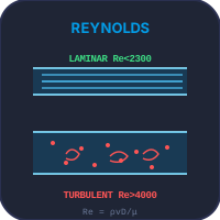
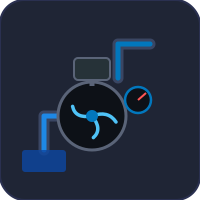
The orifice is one member of a family. Bernoulli's Principle Simulator derives the √(2gH) that this experiment corrects, and shows the same energy bookkeeping in a venturi. Reynolds Number Simulator explains the regime that decides whether these coefficients are constant at all — drop the Reynolds number far enough and Cd stops behaving. Pipe Flow & Pressure Drop continues downstream of the orifice into friction losses in a real line, and Continuity Equation Simulator covers the A×V bookkeeping the contraction coefficient depends on.
Updated