Stefan-Boltzmann Radiation Simulator
P = εσAT⁴ — solve for any unknown, Planck spectrum, T⁴ curve, star & planet • Simulate • Calculate • Explore • Practice • Quiz

Display Controls
Σ Live equations — values substituted
⚖ Temperature scale — P at common T
💡 What-if coach — insights
1 Overview
The Stefan-Boltzmann Simulator visualises the famous T⁴ law: every object hotter than absolute zero radiates electromagnetic energy with power P = ε·σ·A·T⁴. Slide the temperature from 200 K to 6000 K and watch the body change colour from invisible (room T) through dim red (~1000 K), bright orange (~1500 K), yellow-white (~3000 K, light bulb filament), and finally to white-blue near the Sun’s 5800 K.
Built for high-school and technical-college physics students learning thermal radiation, with Practice and Quiz modes for self-testing.
2 Configuring the System

The simulator opens at T = 1500 K (about lava), ε = 0.90, A = 100 cm². Power radiated is P ≈ 2584 W — roughly two and a half kilowatts from a palm-sized surface. Try the Sun Surface preset (5772 K, ε = 1) and P jumps to about 629 kW from that same 100 cm² — 244× more. Raising T by a factor of 3.85 accounts for 3.85⁴ = 220 of that; the remaining 1.11 is the emissivity going from 0.90 to 1.00.
Temperature and area both run on logarithmic sliders, because they span decades: 200 K to 25 000 K, and 0.1 cm² to 5 m². Type an exact value into the box beside either slider when you need one. The Surface dropdown sets ε from a catalogue of real materials (polished silver 0.02 through lampblack 0.95), and Body shape chooses how that surface area is drawn — sphere, cube, or a flat plate radiating from both faces.
3 The Four Canvas Views
The View switch above the canvas changes what is drawn. All four read the same T, ε, A and Tamb.
- Body — the emitting object at true relative size. Its colour is the black-body chromaticity, and its brightness is the real visible-band exitance, so a 1000 K rod looks dim and a 3000 K filament looks blinding. Orange rays leave the surface, blue rays arrive from the surroundings, and a scale bar plus the radius/edge length keep the size mapping honest as the area slider moves across four decades.
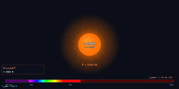
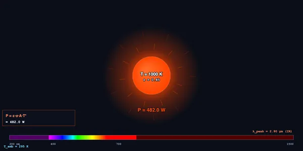
- Spectrum — the live Planck curve Mλ, on a logarithmic wavelength axis from 0.1 to 200 μm. The shaded area under it is εσT⁴, the visible band is painted in real spectral colours, and a grey ghost curve at T/2 shows both the T⁴ drop and the Wien shift in one picture.
- P vs T — the fourth-power curve itself, with a dashed straight line for comparison, your current state marked, and a gold marker at T/2 showing the exact factor-of-16 step.
- Star & Planet — luminosity L = ε·4πR²σT⁴, the flux S = L/4πd² arriving at distance d, and the planet’s equilibrium temperature Teq. Three extra sliders appear — star radius in solar radii, orbital distance in AU, and the planet’s albedo (the fraction of starlight it reflects). The Sun → Earth preset reproduces the 1361 W/m² solar constant and Teq = 254.6 K; seven presets cover the inner planets, Proxima b, Sirius A and Betelgeuse.
Nine readout cards show emitted P, net P, exitance M = P/A, λpeak, the visible fraction, the colour region, T in °C and °F, and P divided by the power the same body would radiate at Tamb. Display Controls (top-left of the canvas) toggle the glow, rays, ambient in-flux, scale bar, equation box and grid. Nine body presets and seven star presets sit above the sliders.
3b Calculate — Solving for Any Unknown
The Calculate tab turns the law around. Pick what you are solving for — Power P, Temperature T, Emissivity ε or Area A — fill in the other three, and press Calculate:
- P = εσAT⁴ · T = (P / εσA)¼ · ε = P / σAT⁴ · A = P / εσT⁴
- Tick Use net radiation and every rearrangement switches to Pnet = εσA(T⁴ − Tamb⁴), with an extra ambient field.
- Temperatures accept K, °C or °F; areas accept m², cm², mm², in² or ft²; power accepts W, kW, mW, MW, BTU/hr or hp.
- Show working prints the full derivation in classical maths notation — and the conversion to kelvin is always its own numbered step, with the size of the error you would have made by skipping it.
- Solving for ε names the closest catalogue surface, and warns if the answer exceeds 1 (which no real surface can).
- Send to simulator loads the solved state back into the Simulate tab.
4 The Underlying Theory
Explore holds 19 concept cards in four categories, and every one of them now carries its own diagram drawn from the same physics engine as the simulator: Basics (why hot things glow, the cavity black body, Wien’s displacement, net vs total radiation), Formulas (Stefan-Boltzmann, Planck’s law, Wien, Kirchhoff and emissivity, T⁴ scaling), Applications (incandescent lamps, infrared thermography, Earth’s energy balance, stellar classification, spacecraft thermal control), Common Errors (kelvin vs Celsius, how steep T⁴ is, area not volume, the grey-body assumption, forgetting the surroundings).
The Learning panels under the simulator hold live equations rendered in classical notation, a reference table of exitance and λpeak at ten standard temperatures, and a what-if coach that reacts to the current state — including how far you are from the Draper point (798 K), the temperature below which nothing glows visibly however hot it is.
5 Try a Problem
Practice generates eight kinds of problem: total power, exitance, Wien’s peak wavelength, the power ratio between two temperatures, a °C-input problem that punishes the Celsius trap, solving backwards for T and for ε, and net radiation against a surrounding temperature. Every one shows real substituted steps — not a generic reminder — and when your answer matches a known mistake (Celsius left unconverted, cm² treated as m², net confused with emitted) the feedback says which mistake you made.
Quiz draws 6 questions at random from a bank of 14, shuffles the options, and explains every answer at the end.
6 Engineering Notes
- Always use absolute temperature in Kelvin! T(K) = T(°C) + 273.15. Plugging Celsius directly gives a wildly wrong answer.
- P scales with T4 — doubling T multiplies P by 16×. Tripling T multiplies P by 81×.
- Net radiation (when in surroundings at Tamb) is Pnet = εσA(T4 − Tamb4). At room temperature your body radiates and absorbs near-equal power.
- Polished metal has very low ε (0.03 for silver). Deliberately poor radiators are used to limit heat loss in vacuum flasks and satellites.
- Below the Draper point (798 K) nothing glows visibly, no matter how much power it radiates. A 700 K plate throws out 13.6 kW/m² and still looks black.
- Emissivity is not a constant of the material — it varies with wavelength, temperature and surface finish. The single-ε grey-body model here is the standard engineering approximation, not the whole truth.
- Units: the SI / Imperial switch converts every displayed value — W becomes BTU/hr, W/m² becomes BTU/(hr·ft²), cm² becomes in², and the °C card becomes °F. Internal calculation stays in SI throughout, and the Imperial choice is remembered across tools. Temperatures on the canvas stay in kelvin, because the law itself is only valid in kelvin.
- Keyboard & mouse: Ctrl+Z / Ctrl+Shift+Z undo and redo, Escape (Esc) closes the calculation modal, Enter submits in Practice and in Calculate, and Right-click on the canvas offers Copy Result, Export CSV, Export PNG and Reset.
- Export: CSV carries the full state plus a 61-point sample of the Planck curve so you can re-plot it in a spreadsheet; PNG saves whichever view is on screen.
- Pair this with the Heat Transfer Modes simulator to compare conduction, convection, and radiation.
Understanding Stefan-Boltzmann Radiation
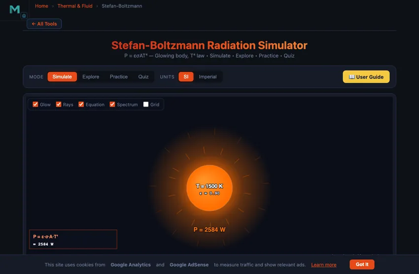
The Stefan-Boltzmann law is the master equation of thermal radiation: every body at absolute temperature T radiates total power P = ε·σ·A·T4, where σ = 5.67×10⁻⁸ W/(m²·K4) is the Stefan-Boltzmann constant, A is the surface area, and ε is emissivity (0–1, 1 = perfect black body).
Power Radiated at Different Temperatures
| Object | T (K) | T (°C) | Flux (W/m²) at ε = 1 | Color |
|---|---|---|---|---|
| Cosmic microwave background | 2.7 | −270 | 3.0×10⁻⁶ | Invisible |
| Frozen ice | 270 | −3 | 301 | Far IR |
| Human body | 310 | 37 | 523 | Far IR |
| Hot iron (dim red) | 1000 | 727 | 56 700 | Dim red |
| Lava | 1500 | 1227 | 287 000 | Bright orange |
| Light bulb filament | 3000 | 2727 | 4.59 MW/m² | Yellow-white |
| Sun surface | 5800 | 5527 | 64.2 MW/m² | White |
| Star (Sirius A) | 10 000 | 9727 | 567 MW/m² | Blue-white |
The T⁴ Power Law
The fourth-power dependence is what makes radiation so dramatic. Doubling temperature gives 16× more power. The Sun’s surface at 5800 K radiates 64.2 MW/m²; at 11 600 K the same surface would radiate 1.03 GW/m². This is also why incandescent lamps are so inefficient: at a 2800 K filament temperature only about 10 % of the radiated power lands in the visible band, and after the eye’s wavelength sensitivity is applied only a few per cent of the electrical energy becomes useful light. Open the Spectrum view at 2800 K and the shaded visible strip shows exactly how little of the curve it covers.
Wien’s Displacement Law
While total power follows T⁴, the peak wavelength of radiation shifts inversely with T: λpeak = 2898 μm·K / T. Cool objects radiate in the infrared (invisible). At ~700 K things start glowing dim red. At ~3000 K (incandescent bulbs) we get yellow-white. The Sun at 5800 K peaks in the green band (which is why our eyes evolved to see green most sensitively!), with broad spread giving white appearance.
Emissivity and Real Surfaces
A perfect black body (ε = 1) absorbs and emits all radiation. Real surfaces have lower emissivity. Polished aluminium has ε ≈ 0.04 — emits only 4% of black-body power. Anodised aluminium 0.77. Human skin 0.98. Soot 0.95. Low-emissivity ("low-E") windows and reflective paints exploit this to limit radiative heat exchange.
Engineering Applications
Incandescent bulbs use tungsten at 3000 K because higher T gives higher visible-light fraction. Infrared thermometers measure T from radiated power and assumed ε. Climate science balances incoming solar radiation against Earth’s outgoing infrared (P_in = P_out). Spacecraft thermal control uses high-ε radiator panels to dump heat into the cold of space, since vacuum eliminates conduction and convection.
The T4 Scaling — Why a 2× Temperature Means 16× Power
The single most important thing about Stefan-Boltzmann is the fourth-power dependence. Double the absolute temperature, the radiated power increases by 24 = 16. Triple it, 81×. This is dramatic and unintuitive.
A practical example: a kitchen oven at 200 °C (473 K) radiates 2840 W/m² from its walls. The same oven at 250 °C (523 K) radiates 4250 W/m² — 50% more power for a 10% temperature rise. This is why oven-cleaning self-cleaning cycles work: heating to 500 °C (773 K) jumps radiated power to 20,200 W/m², which is enough to incinerate grease deposits but obviously requires a sealed cavity.
How the Sun’s Power Reaches Earth — The Full Calculation
This is the calculation that started the field. Sun surface temperature 5778 K. Solar radius 6.96×10⁸ m. Emissivity essentially 1 (close to a perfect blackbody).
| Step | Working | Result |
|---|---|---|
| Solar surface flux | P/A = σT4 = 5.67×10−8 × 57784 | 6.32×10⁷ W/m² |
| Solar surface area | 4πR² = 4π(6.96×10⁸)² | 6.09×10¹⁸ m² |
| Total solar luminosity | P = flux × area | 3.85×1026 W |
| Spread over Earth’s orbit (4πd², d = 1.5×10¹¹ m) | P / (4πd²) | 1361 W/m² |
1361 W/m² is the “solar constant.” Measured by satellites at the top of Earth’s atmosphere; matches the calculation to within 0.1 %. That number is the budget every solar panel, climate model, and crop-growth model on Earth ultimately works from.
Emissivity — Why a Polished Surface Stays Cool
The ε factor in the equation matters as much as T4. Polished metals have ε below 0.1; anodised aluminium around 0.8; oxidised iron 0.85; the human body 0.97. A perfect mirror would have ε = 0 and not radiate at all (it would also reflect everything that hit it).
This is why thermos flasks use silvered inner walls (low emissivity blocks radiation heat transfer), why spacecraft are wrapped in gold foil (reflects sunlight, has low IR emission), and why thermal cameras can detect surface treatments at a glance: a polished area looks “cold” even when it isn’t.
How to Calculate Radiated Power — and How to Run the Law Backwards
Most textbook questions give you three of the four quantities in P = εσAT⁴ and ask for the fourth. All four rearrangements are one line of algebra, and the Calculate tab above performs each of them with the working shown.
| Unknown | Total radiation | Net radiation (surroundings at Tamb) |
|---|---|---|
| Power P | P = εσAT⁴ | Pnet = εσA(T⁴ − Tamb⁴) |
| Temperature T | T = (P / εσA)1/4 | T = (Pnet / εσA + Tamb⁴)1/4 |
| Emissivity ε | ε = P / σAT⁴ | ε = Pnet / σA(T⁴ − Tamb⁴) |
| Area A | A = P / εσT⁴ | A = Pnet / εσ(T⁴ − Tamb⁴) |
Worked example. An oxidised-steel casting (ε = 0.80) with 0.25 m² of surface sits at 450 °C in a 25 °C workshop. How much heat does it actually lose by radiation?
- Convert first: T = 450 + 273.15 = 723.15 K, Tamb = 25 + 273.15 = 298.15 K.
- T⁴ = 2.735×10¹¹ K⁴, Tamb⁴ = 7.903×10⁹ K⁴.
- Pnet = 0.80 × 5.6704×10−8 × 0.25 × (2.735×1011 − 7.903×10⁹) = 3010 W.
- Compare: the emitted term alone is 3100 W, so the surroundings claw back only about 3 %. At 60 °C instead of 450 °C they would claw back 64 %.
Note step 1. Because the law is a fourth power of absolute temperature, entering 450 instead of 723.15 does not produce a small error — it produces an answer 6.7 times too small. Entering 20 instead of 293.15 K is wrong by a factor of 46 000. This is the single most common mistake in the topic, which is why the Calculate tab prints the conversion as a numbered step rather than doing it silently.
Emissivity of Common Surfaces
Emissivity is a property of the surface, not the bulk material: the same steel goes from 0.17 polished to 0.85 oxidised. These are total hemispherical values near room temperature, as used by the Surface dropdown in the simulator.
| Surface | ε | Surface | ε |
|---|---|---|---|
| Black body (ideal) | 1.00 | Concrete | 0.91 |
| Human skin | 0.98 | Oak wood | 0.90 |
| Ice | 0.97 | White paint | 0.90 |
| Matte black paint | 0.96 | Anodised aluminium | 0.82 |
| Water | 0.96 | Steel, oxidised | 0.80 |
| Lampblack / soot | 0.95 | Tungsten filament @2800 K | 0.30 |
| Cast iron, rough | 0.95 | Stainless steel, polished | 0.17 |
| Red brick | 0.93 | Aluminium, polished | 0.04 |
| Glass, smooth | 0.92 | Copper, polished | 0.03 |
| Stainless steel, oxidised | 0.85 | Gold foil / polished silver | 0.02 |
Values from Incropera, Fundamentals of Heat and Mass Transfer 7e Table A.11 and Cengel, Heat and Mass Transfer 5e Table A-18. Treat them as representative: real emissivity varies with wavelength, temperature, oxidation state and surface roughness, sometimes by a factor of two.
Planck’s Law — Where the T⁴ Actually Comes From
Stefan-Boltzmann is not a separate law from Planck’s. It is the area under Planck’s curve. Planck’s spectral radiant exitance gives the power radiated per unit area per unit wavelength:
Mλ(λ,T) = 2πhc² / [ λ5 (ehc/λkT − 1) ]
Integrate that over every wavelength from zero to infinity and the constants collapse into a single number: ∫Mλ dλ = σT⁴, with σ = 2π5k⁴/15h³c² = 5.670374×10⁻⁸ W/(m²·K⁴). Differentiate it instead, set the derivative to zero, and you get Wien’s displacement law. One curve, both results.
The Spectrum view plots that curve live and shades the area under it, so the σT⁴ in the readout and the picture on screen are literally the same quantity. It also integrates the visible band for you: at 1500 K only 0.17 % of the radiated power is visible, at 2800 K about 10 %, and for a 5772 K black body about 46 %. That is why a filament that consumes 60 W of electricity delivers only a few watts of light.
Historically this curve is the reason quantum mechanics exists. Classical physics predicted the exitance would rise without limit as wavelength shortened — the "ultraviolet catastrophe". Planck fixed it in 1900 by assuming energy was emitted in discrete quanta hν, a step he described as an act of desperation. It matched the measurements exactly.
Planetary Equilibrium Temperature
A planet with no internal heat source settles where absorbed starlight equals emitted infrared. Absorbed power is the starlight flux times the planet’s cross-section πRp², reduced by the albedo a; emitted power is σTeq⁴ over the full sphere 4πRp². The planet’s own radius cancels, leaving:
Teq = Tstar · √(Rstar / 2d) · (1 − a)1/4
| Body | d (AU) | Albedo a | Flux S (W/m²) | Teq (K) | Actual mean surface (K) |
|---|---|---|---|---|---|
| Mercury | 0.387 | 0.12 | 9080 | 434 | 440 (day side) |
| Venus | 0.723 | 0.77 | 2600 | 227 | 737 |
| Earth | 1.000 | 0.30 | 1361 | 255 | 288 |
| Mars | 1.524 | 0.25 | 586 | 210 | 210 |
Mars matches almost exactly — its atmosphere is too thin to matter. Earth runs 33 K warm, and Venus runs 510 K warm. Both gaps are the greenhouse effect, and the size of the Venus gap is the clearest evidence in the solar system of what a thick CO₂ atmosphere does. Reproduce every row of this table in the Star & Planet view.
References
- Incropera — Fundamentals of Heat and Mass Transfer, 7th ed., Chapter 12 (Radiation).
- Stefan, J. (1879) — Über die Beziehung zwischen der Wärmestrahlung und der Temperatur. Sitzungsberichte der Akademie. The original derivation.
- NIST — Reference values for emissivity of common materials.
Who Uses This Simulator?
This Stefan-Boltzmann simulator is used by high-school physics students learning thermal radiation, technical-college trainees in heat transfer, mechanical and aerospace engineers sizing thermal radiators, climate-science students modelling planetary energy balance, and astronomy students applying the formula to stars. Practice and Quiz modes ensure students master both the formula and the dramatic T⁴ intuition.
Explore Related Simulators
Explore our Heat Transfer Modes, Thermal Conductivity, Specific Heat Capacity, Phase Change & Latent Heat, and Heat Exchanger, and Thermocouple simulators.
Updated