Stress-Strain Curve Diagram Explained
Hooke's Law • Yield • UTS • Material Properties — Learn • Explore • Practice • Quiz
Display Controls
- Drag the marker along the curve, or use ← → after clicking it
- Display Controls (top-left) switch the construction layers
- Click a name in the diagram’s key to hide that curve
- Click any readout card to see where that number comes from
- Right-click the chart to copy values or export
- Every value in the cards below is measured from the curve on screen
Regions of this curve
Click a region to shade it on the diagram and park the marker inside it. The strain limits shown are read from the model, so they move when you change material.
1 Overview
This is a free, browser-based stress-strain curve simulator for mechanical engineering, materials science and vocational students. Unlike a static textbook figure, the curve here is generated by a calibrated material model — the axes carry real numbers in MPa and strain, and every value in the cards under the diagram is measured back off the curve on screen rather than typed in beside it.
There are five modes:
- Curve — pick a material and press Generate Curve. 23 real materials across three classes, labelled regions, a draggable marker, and every construction an exam asks you to draw. A mild-steel curve is already generated when the page opens.
- Plot My Data — paste your own tensile test and the simulator plots it and extracts E, the 0.2 % proof stress, the UTS, the elongation and the area under the graph.
- Explore — 15 concepts, each with a formula, units and a worked example.
- Practice — 15 randomly generated numeric problems with step-by-step solutions.
- Quiz — 5 questions drawn from a pool of 20, scored with a breakdown.
2 Curve mode — choosing a material
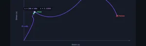
Choosing a curve is a two-step action, on purpose: pick what you want, then press ⚡ Generate Curve at the left of the toolbar under the diagram. Nothing redraws while you are still deciding, so the diagram never changes underneath you mid-sentence. The button lights up whenever there is an outstanding choice, and the line under the dropdowns tells you what is currently on screen.
Generate runs the test. The curve is not simply swapped in — it is plotted from the origin outwards the way a universal testing machine draws it, at a constant strain rate, with a pen tracking the leading edge and crosshairs down to both axes. The specimen above the chart stretches and necks in step with it, the live σ and ε follow the pen, and each landmark label — proportional limit, upper and lower yield, UTS, fracture — only appears at the moment the test actually reaches it. Watching the UTS label appear and then watching the load fall while the specimen keeps stretching is the clearest way to understand why the engineering curve turns over.
Because the pace is a fixed strain rate, a 400 % polypropylene visibly takes longer to break than a 0.07 % ceramic. The test always ends at fracture, so the marker is left at the fracture point; drag it back to inspect anywhere along the curve. A standard mild-steel curve is generated for you as soon as the page loads — without the animation — so there is always something on screen.
The Material and vs dropdowns sit in the toolbar under the diagram, next to the button that uses them, and are grouped by class. 23 materials ship with the tool:
| Class | Materials | What the curves show |
|---|---|---|
| Ductile (15) | Mild steel 1020, ASTM A36, AISI 1045, AISI 4140, 304 stainless, 6061-T6, 1100-O, 2024-T4, copper C11000, brass C26000, Nickel 200, ductile iron 65-45-12, AZ31B magnesium, Inconel 718, Ti-6Al-4V | Yield plateaus (1020, A36) and smooth knees needing the 0.2 % offset; hardening from barely any (6061-T6) to a factor of three (Nickel 200) |
| Brittle (6) | Grey cast iron Class 30 and Class 40, soda-lime glass, alumina ceramic, concrete in tension, PMMA acrylic | Curves with no straight region at all (the irons, concrete, PMMA) and curves that are perfectly straight to the instant of failure (glass, alumina) |
| Polymer (2) | Polypropylene, HDPE | Yield, load drop, cold-draw plateau, then orientation hardening — 400 % and 800 % elongation |
Some pairings are worth generating deliberately. Ductile iron against grey cast iron is the same alloy with the graphite balled up instead of drawn into flakes, and it turns a material that fractures below 0.4 % into one that stretches 12 %. Mild steel, 1045 and 4140 is the strength-versus-ductility trade inside one family. Inconel 718 against mild steel shows 5.5× the strength at identical stiffness — heat treatment and alloying buy strength, never E.
Use the vs dropdown to overlay a second material as a dashed curve on the same axes. Steel against cast iron is the fastest way to see why toughness is not strength. The second curve is never given the material's own colour: two members of one family can be almost the same shade (mild steel and A36 are both violet), so the comparison is drawn in whichever colour from a fixed palette sits furthest from the first. A small key appears at the top-right of the diagram naming both curves — click a name in it to hide that curve and click again to bring it back.
+ Custom material takes five published numbers — E, σy, σu, uniform elongation and elongation at fracture — and calibrates a flow law that passes through all of them at once. If no physical curve can satisfy all five, the tool says so and explains why rather than drawing something plausible.
3 The marker, the specimen and permanent set
Drag the purple marker anywhere along the curve (once the test has finished — the chart is not interactive while the machine is pulling). Click it first and you can also nudge it with the ← and → arrow keys (hold Shift for fine steps, Home and End to jump to either end). Two readout cards follow it: the stress at the marker, and the permanent set that would be left if you unloaded from there.
The specimen drawn above the chart is driven by the same strain as the marker. It stretches by (1 + ε), thins by 1/√(1 + ε) to conserve volume, forms a neck once you pass the UTS, and separates at the fracture strain.
Switch on the Unload line layer to draw the unloading path: a line parallel to the elastic line, back down to the strain axis. Where it lands is the permanent set. Do this once inside the elastic region and once past yield and the difference between "elastic" and "plastic" stops being a definition you memorise.
4 Diagram layers
Every readout card is clickable. Click one and the simulator points at where that number came from on the diagram — the elastic line for E, the peak for the UTS, the shaded triangle for resilience, the whole shaded area for toughness, the marked strain on the axis for elongation. A caption appears explaining what you are looking at. Some quantities genuinely have no place on a stress-strain plot: Poisson’s ratio is a sideways effect, the reduction of area is measured on the broken specimen, and the flow-law exponent is what the curve was generated from rather than something read off it. Those say so and explain how they were obtained instead. The callout stays while your pointer is on the card and fades two seconds after you move away; click the same card again to dismiss it at once.
The small ⓘ button at the top-right of the diagram holds the instructions, the name of what is currently drawn and the note for that material. It is reference text you read once, so it stays folded away rather than taking two permanent rows under the chart.
Display Controls sits on the diagram itself, at the top-left corner — click it to unfold nine checkboxes, and click again to fold it away so it is not covering the chart while you read. On a phone it collapses to a single icon. Everything is on a toggle so you can build the figure up one line at a time, or strip it back to a clean curve before exporting a PNG for a report.
| Layer | What it draws |
|---|---|
| Grid | Gridlines at the axis ticks |
| Key points | Proportional limit, upper/lower yield, UTS and fracture, with leader lines |
| Elastic line (E) | The Hooke line extended, labelled with the fitted modulus |
| 0.2 % offset | The offset construction and its intersection with the curve |
| Elastic zoom | An inset magnifying the first fraction of a per cent of strain, where the elastic region actually lives |
| True σ–ε | The true stress-strain curve, dashed past necking where it is no longer valid without a Bridgman correction |
| Area (toughness) | Shades ∫σ dε under the whole curve, and the resilience triangle inside it |
| Specimen | The tensile specimen, stretching and necking with the marker |
| Unload line | The unloading path from the marker, and the permanent set it leaves |
The elastic zoom is the important one. On an axis that runs to 25 % strain, mild steel’s entire elastic region is 0.125 % wide — half of one pixel. The inset is the only place you can actually see the straight line whose slope is E, and the 0.2 % offset construction crossing it. It hides itself on narrow phones, where there is no room for it.
5 Plot My Data — your own tensile test
Switch to Plot My Data and paste two columns straight out of the UTM software, a CSV or a spreadsheet. Whitespace, commas, tabs and semicolons all work as separators, and header rows are ignored.
- Choose what your columns are: Force (N), Force (kN) or Stress, followed by extension or strain.
- For load columns, enter the original area A₀ and gauge length L₀. The simulator converts to engineering stress and strain for you.
- Press Plot & Analyse.
Strain given as a percentage is detected and converted. In Imperial the columns are read as lbf and inches, and A₀ / L₀ as in² and inches.
Load sample data fills the box with a synthetic 101-point mild-steel test — including a small grip-take-up toe at the origin — so you can see the constructions on a realistic set before committing your own.
The extracted properties appear as cards below the chart, and Show Calculation walks through exactly how each one was obtained. If too few of your points fall inside the straight region, the modulus card is flagged low confidence rather than quietly reported: a modulus fitted to three points is a number, not a measurement.
6 Units, exports and keyboard
The SI / Imperial toggle converts every display: MPa ↔ ksi, GPa ↔ Msi, MJ/m³ ↔ in·lbf/in³, mm ↔ in, mm² ↔ in². The axis is re-rounded in whichever unit you are reading, so the gridlines stay on whole numbers instead of landing on 58.02 ksi. All internal calculation stays in SI; your choice is remembered across the site.
Practice and Quiz problems stay in SI on purpose — they are fixed textbook items, and converting them would put "36.3 ksi" in the question and "250 MPa" in the panel above it.
- CSV and PNG sit at the bottom-right corner of the diagram itself (icons only on a phone). CSV gives the full sampled curve — engineering and true stress and strain, plus a necking flag — with every extracted property in the header comments. PNG gives the labelled diagram at twice screen resolution, watermarked, ready to drop into a lab report.
- Right-click the chart for copy, export, grid toggle and reset.
- Generate Curve re-runs the test at any time, even if nothing has changed.
- Show Calculation opens the full worked derivation in classical notation.
- Keyboard: ← → move the marker, Shift for fine steps, Home / End jump to the ends, Esc closes any dialog.
7 Explore, Practice and Quiz
Explore holds 15 concepts in three categories — Properties, Curve Points and Design. Each shows a diagram drawn from the real material model, a formula, its units, and a worked example. The 0.2 % proof stress card draws the offset construction on the actual 6061-T6 curve, not on a sketch.
Practice generates numeric problems covering stress, strain, modulus, Poisson’s ratio, factor of safety, resilience, required area, elongation, reduction of area, and the true-stress and true-strain conversions. Answers are accepted within ±1 %, and a step-by-step solution is revealed after every attempt.
Quiz draws 5 questions from a pool of 20 — multiple choice and numeric mixed. Options are shuffled every time. The result panel shows your score, a star rating and what you answered for each question.
8 Tips & best practice
- Turn on the elastic zoom first. Most of the confusion about this diagram comes from the fact that everything before yield happens in the first half-percent of the axis.
- Compare mild steel with grey cast iron. Similar order of strength, 270× the toughness. That single overlay is the whole ductile-versus-brittle argument.
- Watch the true curve past the UTS. Switch on True σ–ε and drag the marker past the peak: the engineering curve falls while the true curve keeps climbing. Nothing about the material got weaker.
- Use the unload line to find permanent set before trusting the phrase "elastic limit".
- Units matter: stress in MPa (N/mm²), strain dimensionless, E in GPa, energy per unit volume in MJ/m³ (which is the same number as N·mm/mm³).
- Engineering vs true: this diagram is engineering stress-strain (σ = F/A₀) unless you switch the true curve on.
Understanding Stress-Strain Diagrams — Free Interactive Trainer
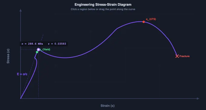
A stress-strain diagram plots engineering stress (σ = F/A0) against engineering strain (ε = ΔL/L0) from a tensile test. It reveals Young’s modulus (elastic slope), yield strength (onset of plastic deformation), ultimate tensile strength (peak stress), and fracture point. The curve shape determines whether a material is ductile or brittle.
The stress-strain diagram is one of the most fundamental tools in mechanical engineering and materials science. It describes how a material responds to applied forces, revealing critical properties such as stiffness, strength, ductility, and toughness. This free interactive trainer lets you explore every region of the curve, study 15 key concepts with formulas and worked examples, and test your knowledge through practice problems and a quiz.
Hooke's Law & the Elastic Region
In the initial linear portion of the curve, Hooke's Law applies: stress is directly proportional to strain (σ = Eε). The slope of this line equals Young's Modulus (E), which measures the material's stiffness. Steel has E ≈ 200 GPa, while aluminium is about 70 GPa. The material returns to its original shape when the load is removed — this is elastic behaviour.
Yield Stress, UTS & Fracture
Beyond the elastic limit, the material begins to deform permanently. The yield stress (σy) marks this transition. For mild steel, a distinct upper and lower yield point is visible. After yielding, strain hardening strengthens the material until it reaches the Ultimate Tensile Stress (UTS) — the peak of the curve. Beyond UTS, necking occurs (a localised reduction in cross-section), and eventually the material fractures.
Ductile vs Brittle Materials
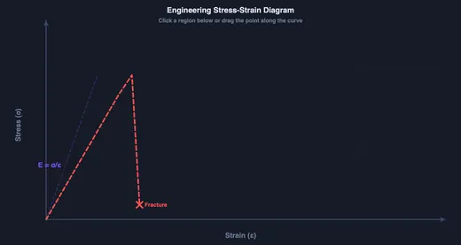
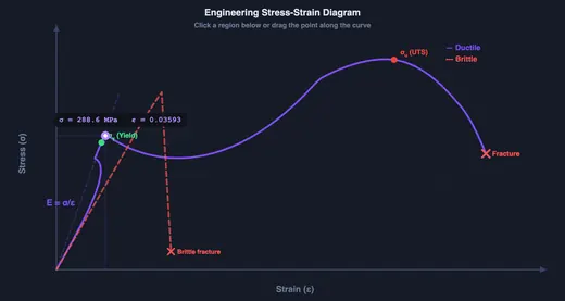
Ductile materials (mild steel, copper, brass, aluminium, titanium) show a long plastic region and a great deal of elongation before fracture. Brittle materials (grey cast iron, glass, ceramics, concrete in tension) fracture suddenly with almost no plastic deformation. Use the vs dropdown to overlay any two of the 23 materials on the same axes: mild steel and grey cast iron are within a factor of two on strength, but the steel absorbs roughly 270 times the energy per unit volume before it breaks. That ratio, not the peak stress, is what "brittle" actually means.
How to Find Young’s Modulus From a Stress-Strain Graph
Young’s modulus is the slope of the straight part of the curve, so E = Δσ / Δε. The practical difficulty is that on an axis running to 25 % strain, that straight part occupies the first 0.125 % — you cannot read a slope off it by eye. Three things make it possible:
- Zoom into the elastic region. Switch on the Elastic zoom layer; the inset magnifies the first fraction of a per cent by a factor of fifty or more.
- Take two points well inside the straight run, not one at the origin. The origin carries the grip take-up — the "toe" — and using it drags the slope down.
- Fit, don’t eyeball. In Plot My Data the simulator locates the straight region by sliding a short chord along your points, keeping the steepest one, and extending over every neighbouring chord still within 1.5 % of it. It then reports the least-squares slope and the R² of that fit.
A fixed rule such as "fit between 10 % and 40 % of the peak stress" looks reasonable and is wrong for any material that yields low against its tensile strength. Annealed copper yields at 69 MPa but peaks at 220, so that window is 22–88 MPa and three quarters of it is already plastic — it returns about 9 GPa for a 117 GPa metal. The straight region has to be found, not assumed.
How to Find Yield Strength and the UTS From a Graph
Yield depends on whether the curve has a knee. Mild steel does: read the upper yield point at the little peak, and the lower yield point on the flat plateau after it — the lower one is the design value. Aluminium, copper, brass and stainless have no knee, so yield is defined by the 0.2 % offset construction described below.
Ultimate tensile strength is the easiest number on the whole diagram: it is simply the highest point of the engineering curve, σu = σmax. It is not an arbitrary peak, though — it sits exactly where Considère’s condition dσtrue/dεtrue = σtrue is met, the point at which strain hardening can no longer keep up with the shrinking cross-section. That is why the strain at the UTS is called the uniform elongation: it is the last strain at which the whole gauge length is still deforming together.
Ductility comes off the horizontal axis: percentage elongation is the strain at fracture × 100, or equivalently (Lf − L₀)/L₀ × 100 measured by fitting the two broken halves back together.
What Is the Area Under a Stress-Strain Graph?
The area under the curve is energy per unit volume. Stress in MPa integrated against a dimensionless strain gives MJ/m³ directly — the units work out because N/mm² × mm/mm is N·mm per mm³. Two areas matter:
- Modulus of resilience, Ur — the triangle under the elastic line only, Ur = ½σyεy = σy²/2E. This is the energy a part can absorb and give back. A spring wants it large, and because it goes as σy squared, strength matters far more than stiffness.
- Toughness, Ut — the whole area to fracture, Ut = ∫σ dε. This needs strength and ductility together.
The gap between them is startling. For mild steel the simulator integrates its own drawn curve and returns Ut ≈ 91 MJ/m³ against Ur = 0.156 MJ/m³ — the elastic triangle is 0.17 % of the total. Almost everything a ductile metal absorbs, it absorbs after it has already yielded. Switch on the Area (toughness) layer to see both shaded at once.
How to Plot a Stress-Strain Graph From Tensile Test Data
If you have a UTM log rather than a textbook curve, use Plot My Data. Paste two columns — load and extension, or stress and strain — give the original area A₀ and gauge length L₀ if you pasted load, and the simulator does the rest:
- σ = F / A₀ and ε = ΔL / L₀ for every row (strain entered as a percentage is detected and converted);
- the curve is plotted with numbered axes and the points that set the modulus highlighted;
- E, the proportional limit, σ0.2, the UTS, the strain at the UTS, the elongation and the area under the graph are all extracted and shown as cards;
- the whole thing exports as a CSV of the data plus properties, or a labelled PNG for a lab report.
This is the step most spreadsheet tutorials skip. Getting a chart out of Excel is easy; getting the 0.2 % offset intersection out of it is not, because the offset line has to be constructed from a slope you first had to fit. Here that construction is drawn on your data, and Show Calculation prints each step with the numbers filled in.
Key Concepts Covered
Explore mode covers 15 concepts: stress, strain, Young’s modulus, Poisson’s ratio, proportional limit, elastic limit, yield stress, ultimate tensile stress, 0.2 % proof stress, necking, factor of safety, resilience, toughness, ductile materials and brittle materials. Each has a formula, its units, a description and a worked example calculation, with the diagram drawn from the same material model as the main curve.
How to Use This Simulator
Start in Curve mode — a mild-steel curve is already generated — switch on the elastic zoom, and drag the marker from the origin to fracture while watching the specimen above the chart and the permanent-set card below it. Then change material and press Generate Curve — the difference between mild steel’s yield plateau and 6061-T6’s smooth knee is the reason two different definitions of yield exist. Use Compare with to overlay a brittle curve. Move to Explore for the formulas behind what you have just seen, then Practice for numeric problems and the Quiz to check yourself. If you have lab data of your own, Plot My Data will analyse it the same way.
Mechanical Properties of Common Engineering Materials
These are the 23 materials the simulator ships with, and the numbers below are the ones the model is calibrated from — the curve you see is generated from this table, not drawn beside it. Uniform elongation is the strain at maximum load (where necking starts); total elongation is the value on the mill certificate. Yield is the lower yield point where the material has a plateau, and the 0.2 % proof stress otherwise.
| Material | E (GPa) | Yield (MPa) | UTS (MPa) | Uniform elong. (%) | Total elong. (%) | ν | Toughness (MJ/m³) |
|---|---|---|---|---|---|---|---|
| Ductile | |||||||
| Mild steel (AISI 1020, hot-rolled) | 200 | 250 | 400 | 20 | 25 | 0.29 | 91 |
| ASTM A36 structural steel | 200 | 250 | 450 | 18 | 23 | 0.29 | 94 |
| AISI 1045 (normalized) | 205 | 379 | 621 | 15 | 21.7 | 0.29 | 126 |
| AISI 4140 (normalized) | 205 | 655 | 1020 | 10 | 17.7 | 0.29 | 169 |
| Stainless steel 304 (annealed) | 193 | 215 | 505 | 35 | 40 | 0.29 | 181 |
| Aluminium 6061-T6 | 69 | 276 | 310 | 9 | 12 | 0.33 | 35 |
| Aluminium 1100-O (annealed) | 69 | 34 | 90 | 32 | 40 | 0.33 | 32 |
| Aluminium 2024-T4 | 73.1 | 324 | 469 | 16 | 20 | 0.33 | 87 |
| Copper C11000 (annealed) | 117 | 69 | 220 | 38 | 45 | 0.34 | 88 |
| Brass C26000 (annealed) | 110 | 95 | 340 | 48 | 55 | 0.35 | 164 |
| Nickel 200 (annealed) | 204 | 148 | 462 | 40 | 47 | 0.31 | 192 |
| Ductile iron 65-45-12 (ASTM A536) | 169 | 310 | 448 | 9 | 12 | 0.29 | 51 |
| Magnesium AZ31B-H24 | 45 | 220 | 290 | 10 | 15 | 0.35 | 41 |
| Inconel 718 (aged) | 200 | 1100 | 1375 | 9 | 12 | 0.29 | 155 |
| Titanium Ti-6Al-4V (annealed) | 114 | 880 | 950 | 10 | 14 | 0.34 | 126 |
| Brittle | |||||||
| Grey cast iron (A48 Class 30) | 100 (tangent) | — | 207 | — | 0.34 | 0.26 | 0.42 |
| Grey cast iron (A48 Class 40) | 128 (tangent) | — | 276 | — | 0.36 | 0.26 | 0.60 |
| Soda-lime glass | 70 | — | 50 | — | 0.071 | 0.22 | 0.018 |
| Alumina ceramic (99.5 %) | 375 | — | 260 | — | 0.069 | 0.22 | 0.090 |
| Concrete (in tension) | 25 (tangent) | — | 3.0 | — | 0.015 | 0.20 | 0.00023 |
| PMMA / acrylic | 3.0 (tangent) | — | 72 | — | 5.0 | 0.37 | 2.3 |
| Polymer | |||||||
| Polypropylene (homopolymer) | 1.5 (initial) | 32 | 42 | — | 400 | 0.42 | 101 |
| HDPE | 1.0 (initial) | 26 | 34 | — | 800 | 0.43 | 172 |
Values are typical and vary with heat treatment, composition, section size and test conditions. Four comparisons in this table are worth generating for yourself:
- Grey cast iron against ductile iron. Chemically almost the same material. Round the graphite into nodules instead of leaving it as flakes and the elongation goes from 0.34 % to 12 %, and the toughness from 0.42 to 51 MJ/m³.
- Mild steel, 1045, 4140. One alloy family, carbon and chromium going up: strength rises from 400 to 1020 MPa, ductility falls from 25 % to 17.7 %, and E never moves off 200–205 GPa.
- Inconel 718 against mild steel. 5.5× the strength at exactly the same 200 GPa stiffness. Strength and stiffness are independent properties.
- Soda-lime glass against anything. 0.018 MJ/m³ of toughness — five thousand times less than mild steel — while being perfectly linear and quite strong right up to the instant it fails.
Key Stress-Strain Formulas
| Property | Formula | Units |
|---|---|---|
| Engineering stress | σ = F / A0 | MPa (N/mm²) |
| Engineering strain | ε = ΔL / L0 | dimensionless (mm/mm) |
| Young’s modulus | E = σ / ε (elastic slope) | GPa |
| True stress | σt = σ(1 + ε) | MPa |
| True strain | εt = ln(1 + ε) | dimensionless |
| Necking (Considère) | dσt/dεt = σt | at σu |
| Permanent set on unloading | εp = ε − σ/E | dimensionless |
| Resilience | Ur = σy² / 2E | MJ/m³ |
| Toughness | Ut = ∫σ dε | MJ/m³ |
| Poisson’s ratio | ν = −εlateral / εaxial | dimensionless |
| Percentage elongation | %El = (Lf − L0) / L0 × 100 | % |
| Factor of safety | FoS = σy / σworking | dimensionless |
Reading a Real Mild-Steel Curve — Five Landmarks That Matter
Pull a tensile specimen of mild steel (low-carbon, ~0.2% C) in the simulator and the curve traces a path no other engineering material draws quite the same way:
- Origin to A — Proportional limit (σpl ≈ 200 MPa). A straight line with slope E (Young’s modulus ≈ 200 GPa). Above this point the stress-strain relation stops being exactly linear, but elastic behaviour persists.
- A to B — Elastic limit (σel ≈ 220 MPa). The largest stress that produces no measurable permanent strain on unloading. In undergraduate practice we treat σpl ≈ σel; in calibration-grade work the difference is microns of permanent strain.
- B to C — Upper and lower yield (σy ≈ 250 MPa). The curve drops slightly, then plateaus and even oscillates — a characteristic of mild steel called yield plateau. The dislocation pile-up at carbon-atom obstacles releases suddenly. This kink is absent in aluminium alloys and stainless steels, which is why those need the 0.2% offset method below.
- C to D — Strain hardening (σ rises to UTS ≈ 400 MPa). Dislocations multiply and entangle, the material gets stronger. The curve climbs but at decreasing slope.
- D to E — Necking and fracture. At UTS, a local cross-section starts to thin (necking). True stress in the neck continues to climb but engineering stress — load divided by original area — falls. The curve descends to fracture at εf ≈ 0.25−0.35 strain (25−35% elongation).
The total area under the curve from origin to fracture is toughness — the energy absorbed per unit volume before failure. For mild steel it is roughly 50−100 MJ/m³. A high-carbon steel of the same UTS but smaller elongation has lower toughness even though it has the same strength.
The 0.2% Offset Method — Defining Yield When the Curve Has No Plateau
Aluminium, brass, copper, stainless steel, and most non-ferrous alloys lack the mild-steel yield plateau — the curve flows smoothly from elastic to plastic with no clear knee. To pin a number to yield strength, engineers use the 0.2% offset method from ASTM E8:
- Draw the elastic line through the origin with slope E (the linear portion of the curve).
- Translate this line to the right by ε = 0.002 (0.2% strain) so it now passes through (0.002, 0) instead of (0, 0).
- The intersection of this offset line with the stress−strain curve is the 0.2% proof stress — the conventional yield strength σ0.2.
For 6061-T6 aluminium, σ0.2 ≈ 276 MPa against a UTS of 310 MPa. Without the offset convention this material would have no “yield strength” at all; with it, it fits into the same design framework as mild steel. Select Aluminium 6061-T6 from the Material dropdown and switch on the Elastic zoom: the offset line is drawn on the real curve, and the value the simulator reports is measured at the intersection rather than looked up — which is why it comes back as the published 276 MPa. Try it on mild steel too. The offset construction lands on 250 MPa there as well, agreeing with the lower yield point you can read straight off the plateau; that agreement is the reason the convention was adopted in the first place.
Ductile, Brittle, Polymer — Three Curve Shapes Side by Side
| Class | Example | Curve shape | Elongation at fracture | Failure mode |
|---|---|---|---|---|
| Ductile metal | Mild steel, aluminium, copper | Elastic line → yield → long plastic plateau → necking → cup-and-cone fracture | 15−40% | Slip on close-packed planes; high toughness |
| Brittle ceramic / cast iron | Grey cast iron, concrete, alumina | Almost linear, fracture before any visible yielding | < 2% | Cleavage on weak planes; very low toughness |
| Thermoplastic polymer | Polypropylene, polyethylene | Non-linear elastic; cold-draw plateau; sometimes strain hardens before tearing | 50−500% | Chain alignment → cold-draw → orientation hardening |
| Elastomer (rubber) | Vulcanised natural rubber | Highly non-linear S-shape; large recoverable strains | 200−600% | Entropic; almost entirely reversible up to fracture |
The same UTS does not imply the same usability. A brittle cast iron at UTS 250 MPa is a poor structural choice because it fails without warning; a ductile mild steel at the same UTS gives visible warning (sag, neck) before fracture. This is why pressure-vessel codes require ductile materials with minimum elongation thresholds.
Common Lab Errors — Why Your UTM Curve Does Not Match the Book
- Wrong gauge length. Elongation depends on gauge length; the standard ratio is L0 = 5.65√A0 (ISO 6892) for proportional specimens. Using L0 = 50 mm on a non-standard specimen gives an “A” value you cannot compare with published data.
- Strain measured from machine crosshead, not extensometer. Crosshead displacement includes machine compliance and grip slip; the apparent E will be 30−50% low. Always use an attached extensometer for elastic-region work.
- Strain rate not controlled. Strain rate affects yield stress: faster pull → higher σy. ASTM E8 specifies 0.015±0.006 mm/mm per minute for the elastic range, with looser control in the plastic range.
- Grip slip mistaken for plastic strain. If the specimen looks loose at the grips after the test, the first part of the curve may be slip not real elongation. Wedge grips with proper bite resolve this.
- Necking ignored in true-stress calculation. Engineering stress falls after UTS, but true stress σtrue = F/Ainstantaneous continues to rise. For metal forming calculations you must convert.
Permanent Set — What Is Left When You Unload
Unloading does not retrace the curve. It follows a straight line parallel to the original elastic line, because only the elastic part of the strain is recoverable. So from any point (σ, ε) on the curve:
- the strain that springs back is εelastic = σ/E;
- what remains is the permanent set, εp = ε − σ/E.
Below the elastic limit εp is zero and the specimen returns to its original length. Above it, the bar is permanently longer. Switch on the Unload line layer and drag the marker: at the UTS of mild steel the tool reports about 20 % permanent set out of 20.2 % total strain — the elastic part is by then almost nothing. This is also the mechanism behind the 0.2 % offset: that construction is nothing more than asking "at what stress would unloading leave 0.002 of permanent strain?"
It is why a spring must stay below yield to be a spring, why a bent sheet stays bent (with a small springback of exactly σ/E), and why cold working raises the yield stress of the metal you have already deformed.
How Accurate Is This Simulator, and Where Does It Stop?
The curve is not a drawing. Up to the ultimate tensile strength it is generated by a flow law fitted in true stress-strain space and calibrated against three conditions at once: it passes through the published yield point, it passes through the published UTS, and it satisfies Considère’s necking condition exactly there. Both a Swift law (σt = K(ε₀ + εp)n) and a Ludwik law (σt = σa + K(εp − εa)n) are available; the readout names which one a given material used. Elastic and plastic strain compose multiplicatively, so the engineering elastic branch is exactly Hooke’s line.
An automated harness re-derives the curve from the shipped source and checks it against more than 5,000 assertions — every material, plus a sweep of 576 user-defined ones. What it verifies:
| Checked | Result |
|---|---|
| Modulus read back off the drawn curve vs the published E | within 0.1 % for all six ductile metals |
| Peak of the drawn curve vs the published UTS | exact for all 23 materials |
| Strain at the peak vs the published uniform elongation | exact — forced by Considère |
| 0.2 % offset construction vs the published yield | within 0.1 % |
| σt = σ(1+ε), εt = ln(1+ε) | at every one of ~630 samples per curve |
| Strain never runs backwards; curve never rises above the elastic line | no violations |
| Round trip: export the curve, re-analyse it as pasted data | recovers E, σ0.2, UTS and toughness |
Where it stops. Three limits are worth stating plainly:
- The branch after the UTS is empirical. The neck geometry is not modelled. That segment is an interpolation from the peak down to the published fracture stress at the published elongation, with zero slope at the peak so the UTS really is the maximum. Everything before the UTS is the calibrated flow law.
- No Bridgman correction. Once necking starts the stress state inside the neck is triaxial, and true stress computed as F/A over-reads. The true curve is therefore drawn dashed past necking, where it is indicative rather than quantitative.
- Rate and temperature are not modelled. Every curve is quasi-static and at room temperature. Yield stress rises with strain rate and falls with temperature; steels have a ductile-to-brittle transition that this diagram cannot show at all.
Grey cast iron and polypropylene have no straight region, so what is labelled E for them is an initial
tangent, and the tool says so on the card. The full record is in
docs/stress-strain-validation.md in the project repository.
Standards and References
- ASTM E8/E8M-21 — Standard Test Methods for Tension Testing of Metallic Materials. The American baseline for tensile tests.
- ISO 6892-1:2019 — Metallic materials — Tensile testing — Part 1: Method of test at room temperature. The international (and European) equivalent.
- IS 1608:2018 — the Indian standard, widely used in Indian polytechnics and aligned with ISO 6892.
- Callister, W. D. — Materials Science and Engineering: An Introduction, 10th ed., Chapter 6 (Mechanical Properties of Metals).
- Dieter, G. E. — Mechanical Metallurgy, 3rd ed., for the true-stress true-strain treatment and the dislocation theory behind yield phenomena.
Explore Related Simulators
If you found this Stress–Strain Curve simulator helpful, explore our Universal Testing Machine simulator, Hooke’s Law simulator, Impact Testing simulator, Mohr’s Circle simulator, Thermal Expansion Calculator, and the Sheet Metal Bend Radius Calculator, where the same ductility that sets elongation also sets the minimum bend radius. The modulus E measured off the elastic slope here is the same E that drives EI in the Beam Bending simulator — stiffer material, shallower deflection curve, identical bending moment diagram. To see the crystal structures behind a metal's strength and ductility, try the Build Your Crystal simulator.
Updated
This form is SI only. Enter the five published properties and the simulator calibrates a flow law that passes through your yield point, your tensile strength and Considère’s necking condition at the same time.