Four Stroke Engine Simulator
Otto & Diesel Cycles — Animate • Learn • Practice • Quiz
Display Controls
Drag the slider, the GAS pedal on the canvas, or press ↑/↓. On the petrol engine the throttle sets manifold pressure: closed, it is the idle-air pressure at which the engine just carries its idle load (about 24–32 kPa, 3.5–4.6 psi, on the petrol presets); wide open, it is the preset’s own value, so a turbo keeps its boost. A diesel has no throttle: its pedal meters the fuel — the heat input qin — from the idle fuelling up to the preset’s own value, and the manifold pressure is never touched. Engine speed follows a stated spool model, I·dω/dt = Tbrake − c·ω² − b·ω, between idle and the rev limiter. The sound is synthesised at the firing frequency, rpm × cylinders / 120.
At wide-open throttle this engine makes no positive brake torque, so it cannot rev above idle. Change the settings or pick a preset.
Live dyno — torque and power against engine speed
Now: — · torque — · power —
Each point is the same air-standard cycle the P–V chart draws, run at that speed. The model has no speed-dependent breathing or friction, so its torque is flat and its power rises in a straight line, P = T·2πN/60. A real engine’s torque peaks in mid-range and falls away as valve flow and friction limit it.
⚙ Engine geometry, breathing & valve timing
Valve timing drives the animated valve lift, the blowdown at EVO and the valve timing diagram. The four ideal state points are still evaluated between BDC and TDC, exactly as the textbook Otto and Diesel cycles are, so the efficiency here always matches the closed-form formula.
Σ Live equations — values substituted from the current engine
📋 Cycle state points — P, V and T at states 1 to 4
⚡ Efficiency breakdown — ideal versus real, and why they differ
💡 What-if coach — insights from the current operating point
1 Overview
The Four Stroke Engine Simulator animates the internal combustion engine through all four strokes — intake, compression, power and exhaust — while solving the air-standard Otto (petrol, spark ignition) or Diesel (compression ignition) cycle behind the picture. Piston, connecting rod and crankshaft are drawn true to scale: the crank radius is half the stroke you type in, the rod is your rod ratio times that, and the bore comes from the bore/stroke ratio. Nothing on the canvas is decorative.
Give it a real engine — bore, stroke, number of cylinders, compression ratio, speed, manifold pressure — and it returns the numbers an engineer actually quotes: IMEP, indicated and brake power, brake torque, BSFC, volumetric efficiency and both the ideal and the realistic efficiency. Three diagrams are available for the same operating point: P–V, T–s and a valve timing diagram.
2 Configuring the Engine

- Cycle — Petrol (Otto) or Diesel. Switching also moves the compression-ratio range (6–14 for petrol, 12–24 for diesel) and resets the air-fuel ratio and heat input to values that suit that cycle.
- Engine preset — six real engine classes: a 125 cc motorcycle, a 2.0 L petrol sedan, a 1.4 L turbo petrol, a 2.0 L TDI diesel, a 6.7 L truck diesel and a 5 kVA diesel genset. Edit any value and the dropdown switches itself to Custom.
- Units — the SI / Imperial toggle converts every readout, every diagram axis and every input box (mm ↔ in, kPa ↔ psi, K ↔ °R, kW ↔ hp, N·m ↔ lbf·ft, g/kWh ↔ lb/hp·h). Every calculation stays in SI internally; only the display changes.
- Engine speed is a real rpm — it drives power, torque and fuel flow. Animation speed is separate and changes only how fast you watch; the readouts always report the rpm you set. Its slider is logarithmic and runs from 3× down to 0.002× — at that setting a 2500 rpm engine takes about 24 seconds per four-stroke cycle, slow enough to follow a single valve opening.
- Compression ratio, heat input qin and manifold pressure set the operating point. Every slider has a companion number box — type an exact value and press Enter.
- Engine geometry, breathing & valve timing (the collapsible panel) holds bore, stroke, cylinder count, con-rod ratio, air-fuel ratio, mechanical efficiency, exhaust back-pressure, intake temperature and the four valve events IVO, IVC, EVO and EVC.
3 Running the Cycle
The engine starts running as soon as the page opens (unless your system is set to reduce motion); Pause / Play stops and restarts it, and it pauses itself while the canvas is scrolled out of view. Step advances exactly one stroke so you can freeze the engine mid-compression and read the state. Reset returns every parameter to its default without stopping or starting the engine. Two keyboard shortcuts work whenever no input box has focus: Space plays and pauses, and S steps one stroke. Esc closes the calculations modal or the right-click menu.
The gas in the cylinder is drawn from the crank angle, so it stays in step with the piston at any animation speed. On the intake stroke fresh charge (blue; pale cyan air on the diesel) grows from the intake valve and pushes the leftover exhaust to the far side; on compression it mixes and warms; the spark starts a flame front that spreads until the burned gas fills the chamber (on the diesel it grows from the bowl the fuel is sprayed into); the burned gas then cools as it expands, rushes out when the exhaust valve cracks open, and is swept out by the rising piston until only the residual is left at TDC. The small tracer dots move with the gas — squeezed and stretched by the piston, entering at the intake valve and leaving at the exhaust valve in the order the gas does. Colour shows temperature. Gas-flow particles also stream in through the intake runner and port, and out through the exhaust port and runner, following the valve lift you set. The spark fires 10° before TDC on the Otto cycle, as a real engine’s ignition advance does; on the Diesel cycle the injector sprays for exactly as long as the constant-pressure burn lasts, so you can watch injection stop at the cutoff point.
The engine is drawn as a section through one cylinder of a twin-cam engine, cut through both valves: oil pan and crankshaft at the bottom, then the piston in its liner with the water jacket around it, then the head with its ports, valves, springs, bucket tappets and two camshafts. A glass runner is clamped to each port, so you can watch the fresh charge drawn in and the exhaust pushed out — and leave the end of the tube as smoke. Each cam lobe is shaped from the same lift curve the valve-timing sliders set and turns at half crank speed, so a lobe presses its valve open only during that valve’s event — watch one lobe make a single turn while the crank makes two. The petrol engine has a pent-roof chamber in the head; the diesel has a flat head and a bowl in the piston crown under the injector. Either way, the space above the piston at TDC is drawn to hold exactly the clearance volume Vc.
The first readout row is the instantaneous cylinder state — stroke, crank angle, pressure, temperature and volume at this instant. The second row is the cycle result and does not change as the crank turns: IMEP, indicated and brake power, torque, BSFC, brake thermal efficiency, peak pressure and temperature, displacement, volumetric efficiency, and (Diesel only) the cutoff ratio.
4 Reading the Three Diagrams
The Diagram selector sits on the top-left of the graph itself — the right-hand pane on a desktop, the lower pane on a phone. Tap P–V, T–s or Valves to switch what that pane draws; the engine cross-section beside it never changes.
- P–V — the pressure-volume trace with the four state points numbered. The volume axis is the real cylinder volume (cm³, or in³ in Imperial) starting from zero, so the strip on the left is the clearance volume. The shaded area is exactly the net work printed beneath it: the green air-standard loop, minus the thin gas-exchange (pumping) loop along the bottom — red when it costs work (throttle the engine down and watch it grow), green when a boosted engine gains from it. Where the trace rounds the corner at state 4, the exhaust valve has opened before BDC (blowdown), giving up a little of the expansion work that the air-standard figure still counts.
- T–s — temperature against entropy. The two vertical lines are the isentropic compression and expansion; the area under 2→3 is the heat added and the area under 4→1 the heat rejected — in kJ/kg, or BTU/lbm in Imperial, where entropy is plotted in BTU/lbm·°R so the areas stay equal to the q values printed under the chart. The ratio of the enclosed area to the area under 2→3 is the thermal efficiency, visible directly.
- Valve Timing — the classical polar diagram with IVO, IVC, EVO and EVC marked and the valve overlap shaded across TDC, plus a valve-lift strip across the full 720°. A live pointer shows where the crank is now.
🎓 Explain, beside Play, Step and Reset, starts a guided lesson written in chalk over the simulator’s own animation while a director camera moves between shots: the whole engine, a close-up of the cylinder, a macro view of the spark plug or injector at ignition, the crankshaft, the valve train and the P–V diagram. It drives the crank itself, so the engine turns through each stroke as it is explained, and every value it writes (clearance and total volume, P1→P2, T1→T2, the heat added, the cut-off ratio, the valve events, the thermal and brake efficiencies) is taken from the engine on screen, in the units you have selected. Change the compression ratio, the fuel, the units or a preset during the lesson and it recalculates in place. Use the controls under the canvas to pause, step between chapters, drag the scrubber, change the lesson speed, or switch the camera from Director to Wide. Space pauses, the arrow keys step and Esc closes it; the current sentence is shown as a subtitle and read out to screen readers. When you close it, the engine is returned exactly as you left it.
Rev it, beside Explain, turns the simulator into an engine you drive. A throttle slider opens under the controls, with a GAS pedal and a tachometer strip on the canvas; drag either, or press ↑/↓, to open and close it. On the petrol engine the throttle sets the manifold pressure; a diesel has no throttle, so on the diesel the pedal meters the fuel (the heat input qin) and the manifold pressure is left alone — whichever control the pedal drives is locked while Rev it is on. Engine speed then follows a stated spool model, brake torque from the cycle against a fan-and-friction load, so it climbs until the load balances the torque or the rev limiter at the preset’s redline cuts in, and falls back to idle when you lift off. The live dyno under it plots brake torque and power across the speed range at the current pedal position, with the operating point marked; the air-standard model has no speed-dependent breathing or friction, so its torque curve is flat. The engine sound is synthesized at the firing frequency, rpm × cylinders / 120: it starts only when you press Rev it, starts muted on a phone, and the sound pill turns it on and off. Turning Rev it off hands back the speed, manifold pressure and heat input it took over.
On a phone the engine and its controls come first: the P–V, T–s and valve-timing diagram is collapsed under the engine so Play, Step and the sliders are within reach. Tap Show diagram to open it (your choice is remembered on that device) and Hide diagram to fold it away again. On a tablet or computer the engine and the diagram sit side by side and nothing is collapsed.
Engine view, the strip above the canvas, switches between 1 cylinder (the sectioned cylinder with its P–V, T–s and valve diagrams, the default) and Multi-cylinder, which puts every cylinder on one crankshaft. The 2 / 4 / 6 / 8 pills set the Cylinders parameter, so displacement, power, torque and the Rev it sound follow; the Cylinders slider works too, from 1 to 12. Inline engines (a 360° parallel twin, inline 3 to 6) are drawn as a side section on the bore centres; V8, V10 and V12 engines as a front view of the V plus each bank seen square to its own deck. Every cylinder runs the same solved cycle, offset by its firing angle, so bore, stroke, rod ratio, compression ratio, valve timing, fuel and speed all act on every cylinder at once. The firing-order timeline shows each cylinder’s four strokes in firing order, with a strip counting how many are on a power stroke, and the torque chart plots each cylinder’s gas torque T = (p − p0)·dV/dθ and their sum: more cylinders, smaller swings relative to the mean (the indicated torque). Friction and the inertia of the moving parts are not included.
3D, the switch beside 1 cylinder and Multi-cylinder in the Engine view strip, shows the engine as a real engine on a training stand: with 1 cylinder chosen, the single cylinder; with Multi-cylinder chosen, the whole engine — a parallel twin, an inline 3 to 6 (or a long inline 7, 9 or 11), or a V8, V10 or V12 — on one crankshaft. It is drawn true to scale from your bore, stroke, rod ratio and compression ratio. Drag to turn it (arrow keys work too), pinch or hold Ctrl and scroll to zoom, and click any part — piston, rings, connecting rod, crankshaft, counterweights, flywheel, valves, springs, camshafts, timing belt, spark plug or injector, water jacket, sump — for a card saying what it does, with live numbers. Cutaway mills away the front-right quarter of the castings and paints the cut faces red, the way a workshop sections a teaching engine; X-ray draws the castings as glass so every moving part shows at once; Exterior shows the engine as it looks from outside. 3/4, Front, Side, Rear and Top move the camera (Rear shows the timing belt, its 18- and 36-tooth sprockets and the flywheel), Labels (off until you turn it on) names the parts in view and Orbit circles the engine slowly. Every cam lobe is cut from the same valve-lift curve the Valves diagram plots, so it touches its bucket at every angle and the cams turn at exactly half crank speed. The charge in the cylinder is coloured by the stroke, the spark (or the diesel spray) appears at the angle the cycle model fires, and the flame grows at the rate the burn model predicts. The card at the top left names the stroke, and the dial at the top right is the 720° cycle: one turn of it is two crank revolutions and one turn of each camshaft. Play, Step, the speed control and every slider drive the 3D engine exactly as they drive the section. On the multi-cylinder engine every cylinder runs the same cycle offset by its firing angle: each crankpin points where its own cylinder needs it, a V’s opposite cylinders share a pin, every camshaft carries one lobe per cylinder turned by half that cylinder’s firing angle, a V has its intakes in the valley under one plenum and its exhausts outboard, and each bank has its own timing belt. The card at the top left then shows the firing order and every cylinder coloured by the stroke it is on. The page opens on the 2D section: press 3D above the canvas to switch, and press it again to come back. The 3D view needs WebGL, which every current browser has.
Display Controls, the matching panel pinned to the top-left of the engine side of the canvas, decides what is drawn: gas-flow particles, TDC/BDC and part labels, the efficiency equation, the diagram grid and the pumping loop. Reset display turns everything back on. On a phone it collapses to a single icon so it never covers the engine.
Right-click (long-press on touch) anywhere on the canvas for a menu: copy the current P, V and T, copy a performance summary, export CSV or PNG, toggle the grid, open the calculations, or reset.
5 Show Calculations, Learning Panels and Export
The calculator icon in the toolbar under the canvas opens a nine-step derivation for the operating point currently on screen, in classical mathematical notation: swept and clearance volume, the trapped charge, isentropic compression, heat addition, expansion, heat rejection and efficiency, mean effective pressure, power and torque, and finally fuel flow, BSFC and brake thermal efficiency. It is rebuilt every time you open it, so it always matches the current engine.
Below the readouts, four learning panels expand and collapse together: Live equations with your numbers substituted, a Cycle state points table of P, V and T at states 1 to 4, an Efficiency breakdown comparing the air-standard, indicated, brake and mechanical efficiencies, and a What-if coach that tells you what would happen if you changed the compression ratio, the heat input or the throttle.
Export CSV, beside it in the same toolbar, writes the full setup, every derived performance figure, the four state points and a 2°-resolution sweep of volume, pressure, temperature and valve lift around the whole 720° cycle — ready to plot in a spreadsheet for a lab report. Export PNG saves the canvas as it stands, watermarked.
6 Practice, Quiz and Explore
Explore holds 23 concept cards across four categories — Fundamentals, Thermodynamic Cycles, Engine Components and Performance — with the equations typeset properly. Practice generates 20 kinds of numerical problem with fresh numbers every time and a worked solution on demand: efficiency for both cycles, swept and clearance volume, MEP, indicated and brake power, torque, BSFC, brake thermal efficiency, friction power, isentropic compression, cutoff ratio, valve overlap and duration, volumetric efficiency and pumping loss. Quiz draws 8 questions from a pool of 26, each with an explanation whether you get it right or wrong.
7 Engineering Notes — What the Model Does and Does Not Do
- The cycle is a cold air-standard cycle. γ = 1.4, cv = 0.718 and cp = 1.005 kJ/kg·K are held constant, the working fluid is air, and combustion is modelled as heat transfer. The efficiency shown always matches the closed-form textbook result exactly — the simulator computes it state by state and the derivation in Show Calculations prints both so you can check.
- State 1 is solved, not assumed. The residual gas left in the clearance volume mixes with the fresh charge, so the temperature at BDC comes out a little above manifold temperature. That is why T1 reads around 320 K rather than 300 K, and it is where the residual gas fraction and the volumetric efficiency come from.
- Why qin is an input rather than something burnt. A stoichiometric petrol charge releases about 3000 kJ per kg of air. Fed into a constant-cv air-standard cycle that would predict a peak temperature near 4900 K, because the model has no dissociation and no rise in specific heat with temperature. Real petrol engines peak at 2500–2800 K. So heat input is set directly, as every textbook gas-power-cycle problem does, and the Efficiency breakdown panel shows what fraction of the fuel's energy that represents.
- Fuel flow comes from the real air-fuel ratio, not from qin. That is what makes BSFC and brake thermal efficiency realistic, and it is why the air-standard efficiency (around 60%) and the brake thermal efficiency (around 25%) are so far apart. That gap — finite burn rate, heat loss to the walls, dissociation, exhaust enthalpy and friction — is the single most important thing this simulator has to teach.
- Valve timing is a gas-exchange model, not a cycle modifier. IVO, IVC, EVO and EVC drive the animated valve lift, the particle flow, the blowdown decay when the exhaust valve cracks open, and the valve timing diagram. The four ideal state points are still evaluated between BDC and TDC, exactly as the textbook Otto and Diesel cycles are, so the efficiency stays checkable against the formula. A late-IVC Miller cycle, where the effective compression ratio really does fall below the geometric one, is described in the Explore cards but is not modelled here.
- Constant-volume combustion overstates peak pressure. Real combustion takes 40–60° of crank, so peak pressure arrives 10–15° after TDC with the piston already descending. The Otto idealisation puts all the heat in at TDC, which is why the peak pressure here runs higher than a real indicator diagram at the same IMEP.
- Volumetric efficiency is the ideal value. There are no flow losses, no intake tuning and no charge heating from the port walls in this model, so it sits near 100% for a naturally aspirated engine. Real engines reach 80–90% at the speed their intake is tuned for and less elsewhere — that shortfall is what shapes the torque curve.
How a Four-Stroke Engine Works — Interactive Simulator
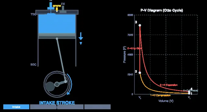
The four-stroke internal combustion engine is the most widely used power source in automobiles, motorcycles, generators, and industrial machinery. Each complete power cycle requires four distinct strokes of the piston—Intake, Compression, Power, and Exhaust—corresponding to two full revolutions (720°) of the crankshaft. This free online engine simulator runs entirely in your browser — nothing to download. It lets you visualise every stroke of a car engine in real time, switch between petrol (Otto cycle) and diesel (Diesel cycle) operation, and enter a real engine — bore, stroke, cylinder count, compression ratio, speed and manifold pressure — to see its pressure, temperature, mean effective pressure, power, torque and fuel consumption. Three linked diagrams share the same operating point: the P–V indicator diagram, the T–s diagram and a valve timing diagram.
Understanding the Otto and Diesel Cycles
In a petrol engine, the Otto cycle governs the thermodynamic process. The air-fuel mixture is compressed isentropically, then ignited by a spark plug at top dead center (TDC), producing a rapid constant-volume pressure rise. The thermal efficiency depends only on the compression ratio: η = 1 − 1/rγ−1, where r is the compression ratio and γ is 1.4 for air. Typical petrol engines operate at compression ratios of 8:1 to 12:1, which gives air-standard efficiencies of 56–63% — roughly double what the engine actually delivers at the crankshaft, for reasons set out further down this page.
The Diesel cycle differs in its heat addition process: air alone is compressed to a high temperature (600–900 K), and fuel is injected under pressure, igniting spontaneously. This constant-pressure combustion introduces the cutoff ratio ρ, making the efficiency formula more complex. Diesel engines use higher compression ratios (14:1 to 22:1) and achieve better fuel economy, though the Diesel cycle efficiency for the same compression ratio is slightly lower than Otto due to the cutoff ratio penalty.
Key Engine Parameters
The compression ratio (r = V1/V2) is the ratio of cylinder volume at bottom dead center to top dead center. Higher compression ratios improve efficiency but increase mechanical stress and require higher octane fuel (petrol) or stronger construction (diesel). The mean effective pressure (MEP) is the constant pressure that, acting on the piston through one stroke, would produce the same net work as the whole cycle — so it measures how hard an engine works independently of its size, and it is directly proportional to torque. Enter a bore, stroke, cylinder count and speed and the simulator returns the swept volume, the trapped charge mass, IMEP and BMEP, indicated and brake power, brake torque, BSFC and volumetric efficiency for that engine.
Reading the PV Diagram
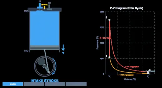
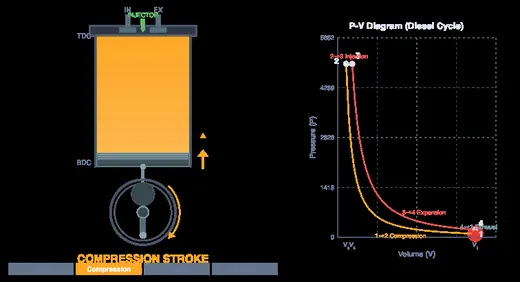
The pressure-volume (PV) diagram shows the thermodynamic state of the gas throughout the cycle. The enclosed area represents the net work output per cycle. In the Otto cycle, you’ll see two vertical lines (constant-volume processes) connected by two isentropic curves. In the Diesel cycle, the upper horizontal line represents the constant-pressure heat addition phase. Watch the PV diagram trace in real time as the piston completes each stroke.
Worked Otto-Cycle Efficiency — A Petrol Engine with Compression Ratio 10
Take a typical naturally-aspirated petrol engine: compression ratio r = 10, working fluid air (γ = 1.4 for the cold-air-standard analysis), intake conditions T1 = 300 K and P1 = 100 kPa, peak temperature T3 = 2000 K. Load the 2.0 L petrol sedan preset and trace it through:
| Step | Process | Working | Result |
|---|---|---|---|
| 1→2 | Isentropic compression: T2 = T1·rγ−1 | 300 × 100.4 | T2 = 754 K |
| 2→3 | Constant-volume heat addition (combustion): qin = cv(T3−T2) | 0.718 × (2000 − 754) | qin = 894 kJ/kg |
| 3→4 | Isentropic expansion: T4 = T3·(1/r)γ−1 | 2000 × 0.10.4 | T4 = 796 K |
| 4→1 | Constant-volume heat rejection: qout = cv(T4−T1) | 0.718 × (796 − 300) | qout = 356 kJ/kg |
| cycle | Thermal efficiency η = 1 − qout/qin | 1 − 356/894 | η = 0.602 (60.2%) |
| shortcut | Otto efficiency: η = 1 − 1/rγ−1 | 1 − 1/100.4 | 0.602 ✓ |
Three lessons drop out: (i) efficiency depends only on compression ratio and γ — not on peak temperature or pressure; (ii) real petrol engines achieve about 30%, not 60%, because of finite heat-release time, exhaust enthalpy loss, friction, and pumping losses; (iii) the only way to raise Otto efficiency is to raise r, which is limited by knock — the point at which the unburnt end gas, compressed further by the advancing flame, reaches its own auto-ignition temperature and goes off on its own after the spark has fired. (Igniting before the spark is a different fault, pre-ignition.) That is why high-octane fuel allows higher compression and therefore higher efficiency.
From Mean Effective Pressure to Power — A Worked 2.0 L Example
Efficiency tells you nothing about how big the engine is. To get from a cycle to a power figure you need the swept volume, the number of cylinders and the speed. Take the simulator’s 2.0 L petrol sedan preset — bore 86 mm, stroke 86 mm, four cylinders, r = 10.5, 2500 rpm, wide-open throttle, qin = 1350 kJ/kg, air-fuel ratio 14.7, mechanical efficiency 0.86:
| Quantity | Working | Result |
|---|---|---|
| Swept volume per cylinder | (π/4)(0.086)²(0.086) | 499.6 cm³ (2.00 L total) |
| Clearance volume | Vs/(r − 1) = 499.6/9.5 | 52.6 cm³ |
| Trapped charge at BDC | p1V1/RT1, T1 = 319 K after mixing with 4.2% residual gas | 0.611 g |
| End of compression | T2 = 319 × 10.50.4; p2 = 101 × 10.51.4 | 817 K, 27.3 bar |
| Peak of combustion | T3 = 817 + 1350/0.718 | 2699 K, 90.0 bar |
| Net work per kg | w = qin − qout = 1350 − 527 | 823 kJ/kg (η = 61.0%) |
| Net work per cycle per cylinder | 0.611 g × 823 kJ/kg | 0.501 kJ |
| IMEP | 0.501 kJ / 499.6 cm³ | 10.03 bar |
| Indicated power | IMEP · Vs · n · N/120 = 1003 × 5.00×10−4 × 4 × 2500/120 | 41.8 kW |
| Brake power and torque | 0.86 × 41.8; then T = 60˙W/2πN | 35.9 kW, 137 N·m |
| Fuel flow and BSFC | 0.586 g air / 14.7 per cycle × 4 cyl × 2500/120 | 11.95 kg/h, 333 g/kWh |
| Brake thermal efficiency | 35.9 kW / (fuel power) | 24.6% |
Two things are worth noticing. The divisor is 120, not 60 — a four-stroke engine fires once every two revolutions, so it makes half as many power strokes per minute as its speed. And the air-standard efficiency of 61.0% has become a brake thermal efficiency of 24.6%: the cycle is not the engine.
Why the Air-Standard Efficiency Is Roughly Double the Real One
Every gas-power-cycle question in a thermodynamics course answers “about 60%” for a petrol engine, and every real petrol engine answers “about 30%”. Both are correct; they are answers to different questions. The air-standard cycle assumes away, in order:
| Assumption | What really happens | Effect on efficiency |
|---|---|---|
| Constant specific heats, no dissociation | cv rises steeply above 1000 K and CO2 and H2O dissociate above ~2000 K, absorbing energy | Large. The cold-air-standard model would predict a 4900 K peak from a stoichiometric charge; the real peak is 2500–2800 K |
| Instantaneous heat addition at TDC | Combustion takes 40–60° of crank; peak pressure arrives 10–15° after TDC | Several points — some of the burn happens while the piston is already descending |
| No heat transfer to the walls | 25–30% of the fuel energy goes into the coolant | Large |
| Exhaust rejected at constant volume | Gas leaves at 700–900 K carrying real enthalpy out of the pipe | Large |
| Frictionless, internally reversible | Piston rings, bearings, valvetrain and the oil and water pumps all take work | 10–25%, captured by the mechanical efficiency |
| No throttling | A part-load petrol engine breathes against a nearly shut plate | Severe at light load — this is the pumping loop on the P–V diagram |
The simulator shows this gap directly. It reports the air-standard efficiency (a function only of compression ratio, and of cutoff ratio for the Diesel cycle) alongside the indicated and brake thermal efficiencies computed from the real air-fuel ratio, and the Efficiency breakdown panel puts all four on the same scale.
Valve Timing, Overlap and the Pumping Loop
The four valve events do not sit neatly at TDC and BDC. A typical naturally-aspirated engine opens the intake about 10–20° before TDC and closes it 40–60° after BDC, exploiting the inertia of the incoming charge; the exhaust opens 40–60° before BDC so that blowdown — gas escaping under its own pressure — drops cylinder pressure before the piston has to push, and closes 10–20° after TDC.
The period around TDC when both valves are open is the valve overlap, equal to IVO + EVC. Wide overlap scavenges the combustion chamber and helps at high speed; it also lets fresh charge escape into the exhaust at idle, which is what gives a big-cam engine its lumpy note. Because a complete cycle is 720° but the cam only needs to open each valve once, the camshaft is geared to run at exactly half crank speed.
Set the manifold pressure below atmospheric in the simulator and watch the bottom of the P–V diagram: the intake stroke now runs below the exhaust stroke, enclosing a second, negative loop. That is pumping work, and its mean effective pressure (PMEP) is subtracted from the gross IMEP every cycle. It is the main reason a petrol engine is inefficient in traffic, and the main reason a diesel — which has no throttle and controls load by injecting less fuel — is not.
The Four Strokes — What Actually Happens Each 720° of Crankshaft
One full cycle of a four-stroke engine takes two crankshaft revolutions (720°). At 3000 rpm that is one cycle every 0.04 s. Press Step in the simulator to advance exactly one stroke at a time and read the cylinder state at each stage:
| Stroke | Piston motion | Valves | What is happening |
|---|---|---|---|
| 1. Intake | TDC → BDC | Intake open, exhaust closed | Cylinder volume grows; atmospheric air-fuel mix is drawn in. Real engines open the intake valve ~10° before TDC for inertial scavenging. |
| 2. Compression | BDC → TDC | Both closed | Mixture is squeezed by ratio r. Temperature rises adiabatically; just before TDC, the spark plug fires (typically 10–30° BTDC). |
| 3. Power (expansion) | TDC → BDC | Both closed | Combustion is complete at ~10° ATDC; the high-pressure gas does work on the piston. This is the only stroke that produces useful torque. |
| 4. Exhaust | BDC → TDC | Intake closed, exhaust open | Burnt gas pushed out. Exhaust valve typically opens ~50° before BDC to let blowdown reduce pumping work. |
The crank-to-cam ratio is 2:1 (the camshaft runs at half engine speed), which is why every other revolution one valve is open. The cam timing diagram is the engineering reality behind the simulator’s Valves diagram, the third setting of the Diagram selector on the graph pane.
125 cc Motorcycle vs 2 L Sedan — Same Cycle, Different Scale
| Parameter | 125 cc motorcycle | 2.0 L sedan |
|---|---|---|
| Displacement (single-cycle volume) | 125 cm³ | 2000 cm³ (typically 4 cylinders × 500 cm³) |
| Compression ratio | 9.5 : 1 | 10.5 : 1 |
| Bore × stroke | 52.4 × 57.8 mm | ~84 × 90 mm per cylinder |
| Peak power | ~11 kW at 8500 rpm | ~110 kW at 6000 rpm |
| Peak torque | ~10 N·m at 6000 rpm | ~190 N·m at 4000 rpm |
| BSFC (brake specific fuel consumption) | ~340 g/kWh | ~250 g/kWh (more efficient combustion at lower rpm) |
The motorcycle makes about 88 kW per litre against the sedan’s 55 — roughly 1.6 times the specific power, bought by spinning 40 % faster — but it pays for it in fuel consumption. Small-engine high-rpm strategies are common where light weight matters more than absolute efficiency.
Otto vs Diesel — Why They Are Different Cycles, Not Just Different Fuels
Set the simulator to Diesel mode and compare the PV diagram. The compression and expansion strokes are essentially the same; the heat-addition (combustion) stroke is the key difference:
- Otto cycle — constant-volume heat addition. Spark ignites a homogeneous air-fuel mixture; combustion completes in roughly 2–3 ms while the piston is near TDC, so volume is approximately constant. The PV diagram shows a near-vertical line at the top.
- Diesel cycle — constant-pressure heat addition. Air is compressed to ~16 : 1; near TDC, fuel is sprayed and auto-ignites. The injection event lasts longer than the spark, so the piston is already moving down while heat is still being added. The PV diagram shows a near-horizontal line at the top.
- Why diesels are more efficient. A higher compression ratio (16–22 vs 9–12 for petrol) gives a higher cold-air-standard efficiency (η ≈ 65% theoretical for Diesel at r=20 vs 60% for Otto at r=10). In practice, diesels deliver ~40% brake efficiency vs ~30% for petrol.
- Why diesels need higher compression. They have no spark plug — fuel must auto-ignite from the heat of compression alone. Air temperature at TDC must exceed about 850 K, which requires r ≥ 14 or so.
Engine Simulator vs Engine Game — What This Simulator Models
Search for an engine simulator and most results are engine games: you rev a car engine, listen to the exhaust note and bolt parts onto a 3D model. This online engine simulator is built for a different job. It calculates what the gas inside the cylinder is doing. Each crank angle is mapped to a state on the air-standard Otto or Diesel cycle. The slider-crank is drawn true to scale, and the P–V, T–s and valve-timing diagrams trace live beside it. Change the compression ratio, bore, stroke, speed or valve timing and the IMEP, power, torque, BSFC and thermal efficiency are recalculated from the cycle, not looked up. Its Rev it mode adds a throttle, a rev limiter and engine sound, but the sound is synthesized from the cycle itself rather than played from a recording, and its 3D view is the same solved engine drawn in three dimensions: the piston, the valves and the cams move by the same laws as the section and the diagrams. Every number on the screen can be checked against a textbook. It runs free in any browser with no download or install, so a student can use it on a school laptop or a phone.
| Feature | This engine simulator | Typical engine game |
|---|---|---|
| Thermodynamic cycle | Air-standard Otto and Diesel cycles, solved state by state | Not modelled |
| Diagrams | Live P–V, T–s and valve-timing diagrams | Usually none |
| Performance outputs | IMEP, BMEP, power, torque, BSFC, thermal and volumetric efficiency | Rpm and a power figure, often cosmetic |
| Mechanism | True-to-scale slider-crank with adjustable valve timing; a multi-cylinder view (twin, inline-3 to 6, V8, V10, V12) with firing order and crankshaft torque; a rotatable 3D cutaway, of one cylinder or the whole engine, whose cams are cut from the valve-lift curve | 3D model, built part by part |
| Sound and revving | Rev it mode: throttle, per-preset rev limiter and engine sound synthesized at the cylinder firing frequency | Main feature |
| Dyno | Live torque and power curve computed from the same cycle | Sometimes, as a game screen |
| Platform | Runs in the browser, free, no install | Often a download or app purchase |
Rev It — Engine Sound, Throttle and a Live Dyno
Press Rev it and the engine simulator becomes something you can drive. Open the throttle with the slider, the GAS pedal on the canvas or the ↑/↓ keys, and the engine speed climbs until the load balances the brake torque or the rev limiter cuts in. Each preset carries its own redline: 10,500 rpm for the 125 cc motorcycle, 6,500 rpm for the 2.0 L sedan and 1.4 L turbo, 4,500 rpm for the 2.0 L TDI diesel, 3,000 rpm for the 6.7 L truck diesel and 1,800 rpm for the diesel generator. On a petrol engine the throttle sets manifold pressure, so a turbo preset keeps its boost at full throttle; a diesel has no throttle, so its pedal meters the fuel instead and the air is never restricted. Sound is off until you press the button, and on a phone it starts muted until you tap Sound on.
How the Engine Sound Frequency Is Calculated
The note you hear is the cylinder firing frequency. In a four-stroke engine each cylinder fires once every two crankshaft revolutions, so
ffire = N × ncyl / 120 (Hz, with N in rpm)
A 4-cylinder engine at 3,000 rpm fires at 3,000 × 4 / 120 = 100 Hz. A single-cylinder motorcycle at 9,000 rpm fires at 9,000 × 1 / 120 = 75 Hz, and a 6-cylinder truck diesel at 2,000 rpm fires at 100 Hz as well. That is why a four and a straight-six can share a pitch at very different engine speeds. The simulator builds the sound from that fundamental and six harmonics, whose loudness follows the indicated mean effective pressure, so the engine sounds harder under load. One- and two-cylinder engines also get a half-order component that gives them their uneven thump. A burst of filtered noise marks each exhaust event, and a filter opens as the throttle opens. No recordings are used: change the cylinder count or the speed and the sound follows the formula.
Reading the Live Dyno
The dyno card sweeps the same air-standard cycle the P–V chart draws across the engine’s speed range at the current throttle, and marks the live operating point. Power and torque are tied by P = T × 2πN / 60: 150 N·m at 3,000 rpm is 150 × 2π × 3,000 / 60 = 47,100 W, or about 47.1 kW. The air-standard model has no speed-dependent breathing or friction, so its torque curve is flat and its power rises in a straight line. A real engine’s torque peaks in the mid-range and falls away as valve flow and friction limit it, which is the gap between the ideal cycle and a measured dyno sheet.
Does This Engine Simulator Have Sound?
Yes. Rev it mode plays engine sound synthesized in your browser from the firing frequency and the cycle’s mean effective pressure. It is off by default, starts only when you press a button, and pauses when you switch tabs. Nothing is downloaded and nothing needs installing.
Multi-Cylinder Engine Simulator — Twin, Inline-4, Inline-6 and V8
Switch the Engine view above the canvas from 1 cylinder to Multi-cylinder and the same engine is shown with every cylinder on one crankshaft. The 2 / 4 / 6 / 8 buttons pick a parallel twin, an inline-4, an inline-6 (straight-six) or a V8, and the Cylinders slider goes from 1 to 12, including an inline-3, inline-5, V10 and V12. Inline engines are drawn as a side section through all the bores, with pistons, connecting rods, crankshaft, camshaft, timing belt and flywheel. V engines are drawn as a front view of the V, showing every crankpin, plus each bank seen square to its deck. Every cylinder runs the same Otto or Diesel cycle the simulator solves, offset by its firing angle, so bore, stroke, compression ratio, rod ratio, valve timing, fuel and rpm change every cylinder at once. It is a free multi-cylinder engine simulator that runs in the browser with no download or sign-up.
Firing Order of 2, 3, 4, 6, 8 and 12 Cylinder Engines
A four-stroke cylinder fires once every 720° of crankshaft rotation, so an engine with n evenly firing cylinders has a power stroke every 720/n degrees. The firing order says which cylinder fires next. The simulator builds the crankshaft from the firing order: each crankpin sits at the cylinder’s firing angle modulo 360°. That gives the flat 180° crank of an inline-4, the three pairs of crankpins 120° apart of an inline-6, and the cross-plane crank of a V8, whose four pins are 90° apart with two connecting rods on each. The torque swing below is for the simulator’s 2.0 L sedan cylinder (86 mm × 86 mm, compression ratio 10.5, 2,500 rpm). It is the peak-to-peak gas torque on the crankshaft divided by its mean.
| Layout | Firing order | Power stroke every | Crankshaft | Cylinders on a power stroke | Torque swing (peak-to-peak ÷ mean) |
|---|---|---|---|---|---|
| Single cylinder | 1 | 720° | One crankpin | 1 for 180°, then none for 540° | 20.7× |
| Parallel twin, 360° crank | 1-2 | 360° | Both pins together | 0 or 1 (360° of every 720° with none) | 10.4× |
| Inline-3 | 1-2-3 | 240° | Three pins 120° apart | 0 or 1 (a 60° gap after each) | 6.9× |
| Inline-4 | 1-3-4-2 | 180° | Flat: 1 & 4 up, 2 & 3 down | Exactly 1, end to end | 5.2× |
| Inline-6 (straight-six) | 1-5-3-6-2-4 | 120° | Pairs 1-6, 2-5, 3-4, 120° apart | 1 or 2 (they overlap) | 3.0× |
| V8, 90°, cross-plane | 1-8-4-3-6-5-7-2 | 90° | Four pins 90° apart, two rods per pin | Always exactly 2 | 2.0× |
| V12, 60° | Even-firing | 60° | Six pins, two rods per pin | Always exactly 3 | 0.8× |
Why More Cylinders Run Smoother
Each cylinder pushes on the crankshaft hard for part of its power stroke and takes torque back while it compresses its charge. The simulator plots that gas torque, T = (p − p0)·dV/dθ, for every cylinder and their sum. With the same cylinder at 2,500 rpm, a single-cylinder engine swings from −182 N·m to +628 N·m around a mean of only 39 N·m, which is why it needs a heavy flywheel. An inline-4 still dips to about −179 N·m between firings, because its power strokes run end to end without overlapping. An inline-6 overlaps them and only dips to about −77 N·m. A V8 never reverses at all: its gas torque stays between +30 and +647 N·m. The mean of the sum is the indicated torque: 156 N·m for the four, 235 N·m for the six and 313 N·m for the V8. That is exactly the number of cylinders times one cylinder’s work per cycle divided by 4π. These curves are gas torque only. The simulator does not model the inertia of the pistons and rods, primary and secondary balance, or vibration, so it shows why more firings smooth the torque, not why an inline-6 is inherently balanced.
Inline-6 vs V8 — What the Simulator Shows
Choose 6 and then 8 to compare the two. The inline-6 fires every 120°, with crankpins in three pairs and firing order 1-5-3-6-2-4. Neighbouring cylinders never fire one after the other, and power strokes overlap for part of each firing interval. The V8 is two banks of four at 90°, with cylinders 1-3-5-7 in one bank and 2-4-6-8 in the other (GM numbering). It fires every 90° on a cross-plane crank, with two connecting rods sharing each crankpin. In the end view you can watch the four pins form a plus sign as the crank turns. Built from the same cylinder, the V8 makes a third more indicated torque, because it has a third more swept volume. Its torque swing also falls from 3.0× to 2.0× of the mean. The firing-order timeline shows the difference directly: the V8 always has two cylinders on a power stroke, while the six alternates between one and two. The engine sound in Rev it mode follows the firing frequency, rpm × cylinders / 120, so at 3,000 rpm a V8 fires 200 times a second and an inline-6 150.
Can I Build My Own Engine in This Simulator?
You can configure one, not assemble one. Choose 1 to 12 cylinders, inline or V, and set the bore, stroke, connecting-rod ratio, compression ratio, intake manifold pressure (boost), valve timing, air–fuel ratio and petrol or diesel combustion. Displacement, power, torque, IMEP, BSFC, efficiency, the firing order and the crankshaft torque all follow from those choices. There is no parts-by-parts assembly; the 3D view shows the engine you configured, cut open, rather than one you build. This is an engine simulator for understanding why an engine makes the power it does, so a V8 here is a set of numbers you can check against a textbook, not a game asset.
3D Engine Simulator — Turn the Engine, Cut It Open, Click Any Part
Press 3D above the canvas and the same engine appears as a real engine on a training stand that you can turn with a finger or the mouse. It is a free 3D engine simulator that runs in the browser: no download, no app and no sign-up. It is not a separate model. It is drawn true to scale from the bore, stroke, connecting-rod ratio and compression ratio you set, and every part moves by the same laws as the section and the P–V diagram. Change a slider and the 3D engine is rebuilt to match: a longer stroke gives a longer crank throw and a taller block, a higher compression ratio a smaller combustion chamber, a diesel a flat head with a bowl in the piston.
Cutaway, X-ray and Exterior Views
Cutaway mills away the front-right quarter of the castings and paints the cut faces red, the way a workshop sections a teaching engine, so the piston, connecting rod, crankshaft, valves and camshafts can be watched working inside a cut section of the block and head. On a multi-cylinder engine the cut runs along the crankshaft, so every cylinder is open at once. X-ray draws the block, head, crankcase and covers as glass, so every moving part shows together. Exterior shows the engine as it looks from outside, with its intake, exhaust, timing belt and flywheel. The camera buttons give a 3/4, front, side, rear (timing belt and flywheel) and top view, and Orbit circles the engine slowly.
Engine Parts and What Each One Does
Click any part in the 3D engine and a card names it, says what it does and gives its live numbers. Labels names every part in view. The parts, and what to watch for in 3D:
| Part | What it does | What to watch in the 3D engine |
|---|---|---|
| Piston and rings | Seals the cylinder and takes the gas pressure on its crown | It stops at TDC and BDC twice per cycle; the flame pushes it down only on the power stroke |
| Connecting rod and gudgeon pin | Turns the piston’s straight-line motion into rotation | The rod swings sideways most at mid-stroke; a shorter rod (lower L/r) swings further |
| Crankshaft | Its crankpin is offset by half the stroke, so one turn moves the piston down and up once | The crankpin circles the main journals; one four-stroke cycle takes two turns (720°) |
| Counterweights | Balance the rotating mass of the crankpin and the big end of the rod | The heavy lobe is always opposite the crankpin |
| Flywheel and ring gear | Stores energy from the power stroke to carry the engine through the other three | One cylinder fires once every two turns; the flywheel is what keeps it turning between firings |
| Cylinder and water jacket | The bore the piston slides in, with coolant passages around it | In the cutaway the jacket shows as a passage around the bore wall |
| Cylinder head and combustion chamber | Closes the cylinder; the chamber is the clearance volume Vc | A petrol head has a pent roof; a diesel head is flat with a bowl in the piston crown |
| Intake and exhaust valves | Let the charge in and the burnt gas out | The intake valve is the larger one; around TDC both are slightly open (valve overlap) |
| Valve springs and bucket tappets | Close each valve and keep it following its cam | Each spring compresses as its valve opens |
| Camshafts | Each lobe is shaped to open a valve by the right amount at the right time | The camshafts turn at exactly half crank speed; each lobe touches its bucket at every angle |
| Timing belt and sprockets | Keep the valves in step with the piston | The cam sprockets have 36 teeth and the crank sprocket 18: the 2 : 1 drive (Rear view) |
| Spark plug or fuel injector | Starts combustion: a spark in a petrol engine, a fuel spray into hot air in a diesel | The spark flashes a few degrees before TDC; the diesel injector sprays six plumes just before TDC |
| Throttle body | On a petrol engine, sets the load by restricting the air | The butterfly opens as you raise the manifold pressure; a diesel has none |
V8, Inline-6 and Parallel Twin Engines in 3D
Choose Multi-cylinder as well as 3D and the whole engine is drawn on one crankshaft: a parallel twin, an inline-3 to inline-6, or a V8, V10 or V12. Each cylinder runs the same cycle offset by its firing angle, so the card above the engine shows the firing order and colours every cylinder by the stroke it is on. In a V8 the two cylinders opposite each other in the V share one crankpin, the intakes sit in the valley under one plenum, the exhausts run outboard and each bank has its own timing belt. Every camshaft carries one lobe per cylinder, turned by half that cylinder’s firing angle, which is how one shaft opens every valve in the firing order.
Is There a Free 3D Engine Simulator Online?
Yes. This engine simulator has a 3D view that runs free in any current browser, on a computer, tablet or phone, with nothing to download or install. It needs WebGL, which every current browser has. It is built for understanding how an engine works rather than for driving or building one: what you see in 3D is the same Otto or Diesel cycle the simulator solves, with the same valve timing, the same piston motion and the same burn.
Selected References
- Heywood, J. B. — Internal Combustion Engine Fundamentals, 2nd ed., McGraw-Hill, Chapters 1, 5 and 9. The definitive engineering text for IC engines.
- Cengel, Y. A. & Boles, M. A. — Thermodynamics: An Engineering Approach, 9th ed., Chapter 9 (Gas Power Cycles).
- SAE J1995 — Engine Power Test Code — Spark Ignition and Compression Ignition — Gross Power Rating. Defines the conditions under which an engine’s “peak power” spec must be measured.
- ISO 1585 — Road vehicles — Engine test code — Net power. The European equivalent.
Explore Related Simulators
If you found this four-stroke engine simulator helpful, explore our Two Stroke Engine Simulator, Thermodynamics Simulator, Heat Transfer Simulator, and Stress-Strain Diagram for more hands-on practice. To measure what an engine actually delivers rather than what the air-standard cycle predicts, the Morse Test simulator separates indicated power from friction losses on a multi-cylinder engine.
Updated