Why Fatigue Failure Surprises Engineering Students — And How I Fixed That

Static failure is intuitive. Apply enough force to a bar of steel and it yields, then fractures. Every student understands the logic: too much stress, something breaks. Textbooks teach it first because it’s the simplest story to tell.

Fatigue failure is a different kind of surprise entirely. A crankshaft spins through millions of cycles at a stress well below the yield point. Weeks pass. Then it snaps — suddenly, with no warning, at a stress that wouldn’t dent a static specimen. Students hear this and don’t quite believe it. The numbers don’t match their mental model. The material didn’t “fail” by the rules they learned.

That disconnect is exactly where I used to lose them. The theory is correct; the intuition just hasn’t been built yet. And drawing S-N curves on a whiteboard doesn’t build it. You need to work the numbers across several materials, adjust the parameters, and see the life estimate change in real time. That’s what the Fatigue Life Simulator does — and this article walks through how I use it across a full fatigue unit.

The Problem With Teaching Fatigue From Textbooks

Here’s the core difficulty: fatigue is a statistical, microscopic, progressive phenomenon being described by macroscopic engineering equations. The gap between “a crack is nucleating at a grain boundary” and “σ_a/S_e + σ_m/S_ut = 1/n” is enormous, and most introductory courses skip over it.

What students end up with is a set of formulas they can apply but not picture. They know there’s a “fatigue limit” and they know steels have one while aluminium doesn’t, but they can’t tell you why the S-N curve bends flat at 10⁶ cycles for steel and keeps dropping for aluminium alloys. They know Goodman is “the one you use” but not how it differs from Soderberg, and why anyone would choose Gerber instead.

The other problem is numbers. Fatigue is a log-log world — a change from 10⁵ to 10⁶ cycles sounds small but represents a tenfold increase in life. Students raised on linear graphs struggle to read S-N curves correctly. They interpolate linearly where they should be working in log space. A fatigue life calculator that plots in real log-log scale, with a live operating point they can drag, fixes that reading problem in a single session.

Understanding the S-N Curve: Basquin’s Equation Made Visible

The S-N curve (also called a Wöhler curve) plots stress amplitude σ_a against number of cycles to failure N on a log-log scale. The underlying relationship is Basquin’s equation:

\[\sigma_a = \sigma'_f \left(2N\right)^b\]

where σ′_f is the fatigue strength coefficient (related to the true fracture strength) and b is the fatigue strength exponent — negative, because stress amplitude must decrease as life increases. For most steels, b sits between −0.07 and −0.12. Flatter b means the material retains fatigue strength well; steeper b means life drops quickly as stress rises.

For Steel 4140 (S_ut = 1020 MPa), the Shigley data gives σ′_f = 1580 MPa and b = −0.085. At N = 10⁶ cycles that works out to:

\[\sigma_a = 1580 \times \left(2 \times 10^6\right)^{-0.085} = 437 \text{ MPa}\]

That’s the stress amplitude at which you’d expect one million cycles. The true endurance limit for ferrous materials is defined at 10⁶–10⁷ cycles (Shigley uses 10⁶ for high-strength steels). Below S_e′, infinite life is assumed. The standard estimate for steels with S_ut ≤ 1400 MPa is:

\[S'_e = 0.5 \times S_{ut} \quad (\text{for } S_{ut} \leq 1400 \text{ MPa})\]

For Steel 1020 (S_ut = 395 MPa), that gives S_e′ = 197.5 MPa. Simple. But for Al 6061-T6 (S_ut = 310 MPa) there’s no horizontal knee in the S-N curve at all. Aluminium and most non-ferrous alloys don’t have a true endurance limit — the curve keeps descending. A finite design life (typically 5 × 10⁸ cycles) is chosen instead. Showing students both curves on the same plot, side-by-side, instantly communicates why aluminium aircraft components need careful life tracking while steel springs can be designed for infinite life.

To solve for life at a given stress amplitude, you invert Basquin’s equation:

\[N = \dfrac{1}{2}\left(\dfrac{\sigma_a}{\sigma'_f}\right)^{1/b}\]

The 1/b exponent is large and negative (for b = −0.085, it’s roughly −11.8). That’s why fatigue life is so sensitive to stress amplitude. A 10% increase in σ_a doesn’t reduce life by 10% — it can cut it in half.

Marin Factors: Why Your Lab Sample and Your Real Part Behave Differently

The endurance limit S_e′ is measured in a controlled lab environment on a polished, 7.5 mm rotating-beam specimen at room temperature with 50% reliability. Your actual part is none of those things. It’s bigger, machined with a real surface finish, operating at a real temperature, with stress concentrations at every shoulder and keyway. That’s where the Marin equation comes in:

\[S_e = k_a \cdot k_b \cdot k_c \cdot k_d \cdot k_e \cdot S'_e\]

Each factor accounts for one way the real part differs from the test specimen. Let’s take Steel 4140 (S_ut = 1020 MPa) through all five:

k_a — Surface finish. The Marin surface factor for a machined surface on 1020 MPa steel is k_a = 4.51 × 1020^−0.265 ≈ 0.82. A ground surface gives k_a closer to 0.93; a forged surface can be as low as 0.57. Surface finish is usually the biggest single derating factor because fatigue cracks initiate at surface irregularities.

k_b — Size. Larger parts have a higher probability of containing a critical flaw in the highly stressed volume. For a solid 40 mm shaft, k_b ≈ 0.85. For a 10 mm shaft, k_b = 1.0.

k_c — Reliability. At 50% reliability, k_c = 1.0. At 99% reliability, k_c = 0.814. At 99.9%, k_c = 0.753. Most engineering designs use 90% (k_c = 0.897) or 99%.

k_d — Temperature. At room temperature, k_d = 1.0. For elevated-temperature applications above 450°C, fatigue strength drops and k_d < 1.0. This matters for exhaust components, turbine parts, and anything near a combustion chamber.

k_e — Stress concentration. This is often the most severe factor. k_e = 1/K_f, where K_f = 1 + q(K_t − 1). K_t is the theoretical geometric stress concentration factor; q is the notch sensitivity of the material (0 to 1, higher for stronger materials). A sharp shoulder fillet on a 4140 shaft might give K_t = 2.5 and q ≈ 0.95, so K_f ≈ 2.43 and k_e ≈ 0.41. That alone cuts the endurance limit by more than half.

Students consistently underestimate how much these factors stack. Running through a worked example on the simulator — watching S_e drop from 510 MPa to something around 180 MPa after all five corrections — lands harder than any table in a textbook.

The Goodman Diagram: When Mean Stress Gets Involved

Up to this point, all the analysis assumes fully-reversed loading — a stress cycle that swings equally between tension and compression, with zero mean stress. Real components almost never load that cleanly. A rotating shaft in bending comes close, but add a press-fit hub, a preloaded bolt, or a residual stress from heat treatment, and you have a non-zero mean stress σ_m sitting on top of the alternating amplitude σ_a.

Mean stress changes everything. Tensile mean stress accelerates crack propagation and shortens fatigue life. The Goodman diagram captures this with a failure line across the σ_m–σ_a plane. The modified Goodman criterion is:

\[\dfrac{\sigma_a}{S_e} + \dfrac{\sigma_m}{S_{ut}} = \dfrac{1}{n}\]

where n is the safety factor. For a crankshaft bearing journal with σ_a = 150 MPa, σ_m = 50 MPa, S_e = 217 MPa (corrected), and S_ut = 1020 MPa:

\[n = \left(\dfrac{150}{217} + \dfrac{50}{1020}\right)^{-1} \approx 1.35\]

A safety factor of 1.35 against the Goodman line. Whether that’s acceptable depends on the consequences of failure. For an aircraft component you’d want n ≥ 1.5 minimum; for a general industrial part, 1.2–1.5 is often acceptable.

The three criteria differ in how they draw that failure boundary:

• Goodman — linear from (0, S_e) to (S_ut, 0). The standard for industry. Conservative enough for most steels, straightforward to apply.
• Soderberg — linear from (0, S_e) to (S_y, 0). More conservative because S_y < S_ut. Guarantees that yielding won’t occur before fatigue failure. Use this where plastic deformation is completely unacceptable.
• Gerber — parabolic: (σ_m/S_ut)² term. Fits experimental ductile-steel data most accurately but is unconservative at high mean stress. Useful for academic comparison; less common in design codes.

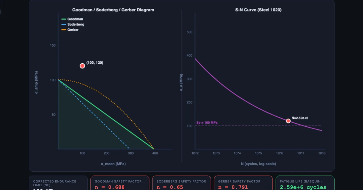
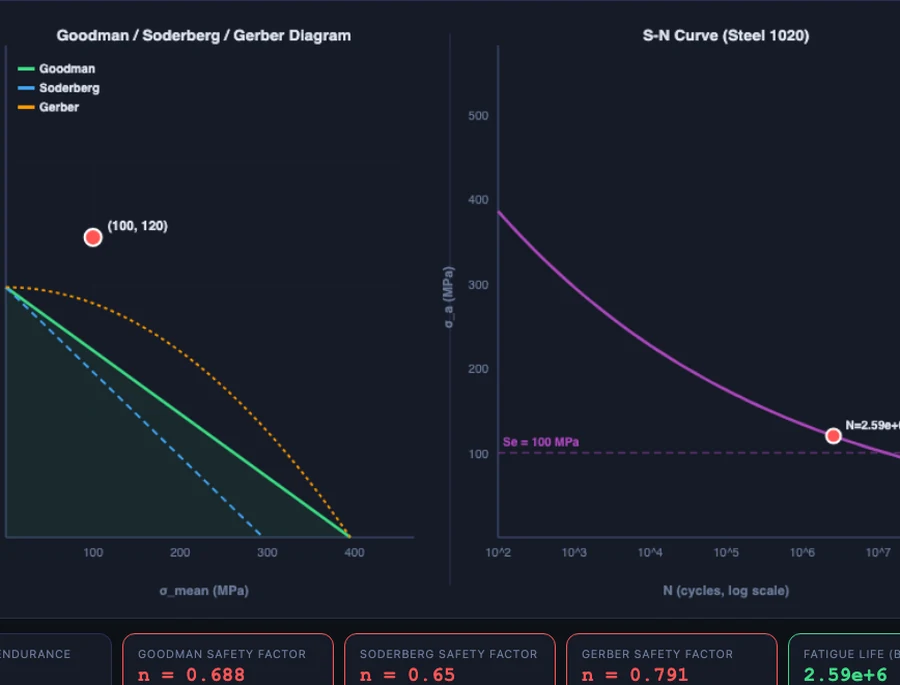
The body image above shows all three plotted simultaneously for the crankshaft scenario. The operating point (150, 50) sits inside the Goodman boundary (safe) with n ≈ 1.35, well inside Soderberg (safer), and comfortably inside Gerber. Seeing the three lines around a single point immediately communicates how much the choice of criterion shifts the apparent safety margin — without requiring a single additional word of explanation.

How I Structure the Fatigue Unit in My Class

I’ve tried several orderings over the years and landed on a four-stage progression that maps directly to the simulator’s features.

Stage 1: S-N curve first, formulas second. Before any equations, students open the simulator and select two materials — I usually start with Steel 4140 and Al 6061-T6. They look at the curves and I ask three questions: Which material would you choose for a part that spins a billion times? Which one drops in strength faster? What’s the stress amplitude at 10⁶ cycles for each? They work out the answers from the graph. Then I introduce Basquin’s equation as the formula that describes the curve they’ve already seen. The formula lands completely differently when you’ve seen the curve first.

Stage 2: Marin factors as a checklist. I give students a scenario — a machined 4140 crankshaft, 40 mm diameter, 99% reliability, operating at room temperature, with a fillet K_t = 1.8. They work through k_a through k_e one by one, entering each factor into the simulator as they go and watching S_e drop. By the end, the corrected endurance limit is usually around 170–190 MPa instead of the raw 510 MPa. That factor-of-three reduction is a genuine shock to most students.

Stage 3: Goodman diagram for design problems. Once they have S_e corrected, the Goodman diagram becomes a design check. I give a loading scenario (alternating and mean stress from a combined bending-torsion case using the Shaft Torsion Simulator), and they plot the operating point, read off the safety factor, and decide if it’s acceptable. Then I ask: what if we wanted n = 2? How would you redesign?

Stage 4: Design project. Students choose a rotating component (shaft, crankshaft, connecting rod, axle) and do a full fatigue analysis: material selection, Marin correction, loading analysis, Goodman check. They have to defend their material choice and show that the safety factor is appropriate for the application. The simulator is their calculation tool throughout; the report explains the engineering decisions. It’s the one assessment task where students consistently say they understood what they were doing while they were doing it — not in retrospect.

For more on combining bending and torsion before a fatigue check, the shaft torsion formula guide covers the polar moment of inertia and shear stress distribution in detail. And for the material side of things, the stress-strain curve guide explains where S_ut and S_y come from in the first place.