Spring-Mass-Damper Vibrations Simulator — Natural Frequency, Damping & Resonance

Every car ride you've ever taken was shaped by a spring-mass-damper system. The spring-mass-damper vibration simulator lets you change mass, stiffness, and damping in real time, watch the oscillation on a live waveform, and immediately see how natural frequency and damping ratio respond. It's one of those rare tools where the theory and the behaviour snap into alignment the moment you move a slider.

Why students get confused about vibrations

Here's a pattern I see every semester. The student can write down ω_n = √(k/m) without a second thought. Ask them what happens when you double the mass — they'll tell you the frequency drops. Fine. Then ask what happens to the damped frequency when you increase damping near the critical value, and the room goes quiet.

The trouble isn't the formula. It's that vibration concepts — natural frequency, damping ratio, resonance, transmissibility — all interact in ways that are hard to track on paper. The system is underdamped, so it oscillates. But how fast does the oscillation die? And what happens if you add a forcing frequency that matches ω_n? Those aren't questions a static diagram answers well.

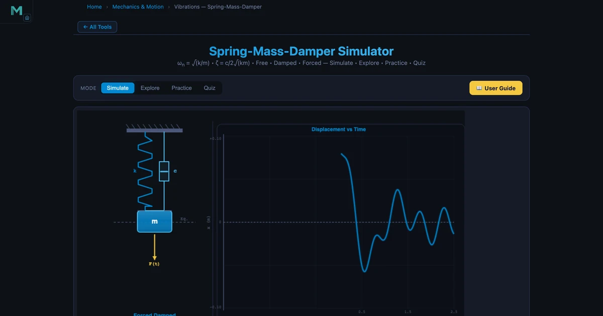
The simulator shows all four vibration types — free undamped, free damped, forced undamped, and forced damped — with a live animated spring-mass-damper on the canvas and a scrolling waveform chart. The readout cards update instantly as you move the sliders. That feedback loop is what the textbook can't give you.

The core formulas — what each number actually means

The equation of motion for a forced damped system is:

\[m\ddot{x} + c\dot{x} + kx = F_0 \sin(\omega t)\]

Three parameters define the system entirely: mass \(m\) (kg), spring stiffness \(k\) (N/m), and damping coefficient \(c\) (Ns/m). From these, two non-dimensional quantities govern the response:

\[\omega_n = \sqrt{\dfrac{k}{m}} \quad \text{(natural frequency, rad/s)}\]

\[\zeta = \dfrac{c}{2\sqrt{km}} = \dfrac{c}{2m\omega_n} \quad \text{(damping ratio)}\]

In the Car Suspension preset, k = 500 N/m and m = 20 kg, so ω_n = √(500/20) = 5.00 rad/s. With c = 50 Ns/m, the critical damping is c_c = 2√(km) = 2√(10000) = 200 Ns/m, giving ζ = 50/200 = 0.250. That's a lightly underdamped system — realistic for a passenger vehicle suspension.

For forced vibration, the steady-state amplitude depends on the frequency ratio \(r = \omega / \omega_n\) and the magnification factor:

\[M = \dfrac{1}{\sqrt{(1 - r^2)^2 + (2\zeta r)^2}}\]

The Car Suspension is forced at 2 Hz, giving ω = 2 × 2π = 4π rad/s. The frequency ratio r = 4π/5 = 2.513. Plugging into M: with r = 2.513 and ζ = 0.250, M ≈ 0.183 — the suspension actually reduces the forcing amplitude, because the system operates well above resonance (r > √2 ≈ 1.414). The simulator confirms: amplitude = 0.0183 m = M × (F₀/k) = 0.183 × (50/500).

The four simulation presets and what they teach

Car Suspension — damped forced vibration

This is the most practically grounded preset. A 20 kg quarter-car mass on a 500 N/m spring with 50 Ns/m damping, forced at 2 Hz (road undulations). The key lesson: with r = 2.513 and ζ = 0.25, the system is deep in the isolation zone. The amplitude is only 18.3 mm. Students are surprised — softer springs actually absorb road vibrations better because they push the natural frequency below the excitation. The real challenge in suspension design is keeping ζ high enough (ride comfort) without reducing the isolation too much.

Tuning Fork — free damped vibration

Mass 0.5 kg, k = 500 N/m, c = 0.1 Ns/m. Natural frequency ω_n = √(500/0.5) = 31.62 rad/s ≈ 5.03 Hz. Damping ratio ζ = 0.1/(2√(500×0.5)) = 0.1/20 = 0.005 — essentially undamped. The waveform shows hundreds of oscillations before amplitude visibly decays. This illustrates logarithmic decrement: δ = 2πζ/√(1−ζ²) ≈ 0.031, meaning each successive peak is only 3.1% smaller than the previous one.

Bridge Resonance — undamped forced near resonance

m = 20 kg, k = 200 N/m, c = 1 Ns/m. The forcing frequency is set equal to the natural frequency — r = 1. With such low damping (ζ = 0.009), the amplitude magnification factor M = 1/(2ζ) = 56. The waveform grows wildly. This is the Tacoma Narrows Bridge scenario from 1940, where wind-induced oscillations near the bridge's natural frequency drove the amplitude to failure. Engineers use this preset to make the point visceral: resonance isn't just a theoretical edge case. It kills structures.

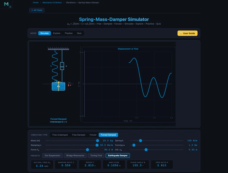
Earthquake Damper — heavily damped forced vibration

m = 20 kg, k = 100 N/m, c = 50 Ns/m, forcing at 1 Hz. Natural frequency ω_n = √(100/20) = 2.24 rad/s, ζ = 50/(2√2000) = 50/89.4 = 0.559. The frequency ratio r = (1 × 2π)/2.24 = 2.810. Amplitude = 0.1056 m. Despite operating above resonance with significant forcing, the heavy damping keeps the amplitude controlled. This is the operating principle of tuned mass dampers in tall buildings — Taipei 101's 730-tonne pendulum uses exactly this approach.

Worked example — verifying the damped natural frequency

For the Earthquake Damper preset, the damped natural frequency is:

\[\omega_d = \omega_n \sqrt{1 - \zeta^2} = 2.24\sqrt{1 - 0.559^2} = 2.24\sqrt{0.687} = 2.24 \times 0.829 = 1.857 \text{ rad/s}\]

The free-damped oscillation follows:

\[x(t) = A_0 e^{-\zeta \omega_n t} \cos(\omega_d t + \phi)\]

The exponential envelope decays with time constant τ = 1/(ζω_n) = 1/(0.559 × 2.24) = 0.797 s. After one second, the amplitude has dropped to e^−1.254 ≈ 28.5% of its initial value. That's fast — within 3–4 seconds, the free oscillation is essentially gone. The phase angle for forced vibration is φ = arctan(2ζr/(1−r²)). With r = 2.810 and ζ = 0.559: numerator = 2 × 0.559 × 2.810 = 3.143, denominator = 1 − 7.896 = −6.896. Since the denominator is negative, φ is in the second quadrant: φ ≈ 155.5°. The simulator readout confirms this exactly.

How to use this in a lesson

Opening hook (5 min). Show the Bridge Resonance preset with no explanation. Let the waveform fill the screen and watch the amplitude grow. Ask: "What's causing this?" Students will offer guesses. Let them debate briefly before revealing the concept of resonance. It lands differently when they've seen the number explode in front of them.

Core concept pass (15 min). Walk through the four presets in order: Free Undamped → Free Damped → Forced → Forced Damped. At each step, ask students to predict what changes before you apply the preset. The forced damped session benefits from comparing r < 1, r = 1, and r > 1 by manually dragging the forcing frequency slider.

Design challenge (10 min). Give students a target: design a mount (choose k and c) for a machine running at 3000 RPM (ω = 314 rad/s) that gives transmissibility TR < 0.1. They need to pick ω_n < ω/√2 and check TR = √((1+(2ζr)²)/((1−r²)²+(2ζr)²)). The simulator lets them verify their design instantly — no derivation required to check the result. This connects to the SHM simulator guide where similar mass-spring concepts are explored.

Explore mode wrap-up (5 min). Switch to Explore mode and walk through the transmissibility concept card. The graph showing TR vs r for different ζ values crystallises why low-damping mounts are preferred above r = √2 — something that surprises most students the first time they see it.