The Number That Breaks Shafts: How I Teach Stress Concentration With a Simulator

My students are competent at calculating nominal stress. Hand them a bar with a rectangular cross-section and an axial load and they’ll give you σ = F/A without hesitation. They’ve drilled it. They trust it. And that confidence is exactly the problem.

Real parts aren’t featureless bars. They have holes for fasteners, keyways for drive components, fillets where one diameter steps to another. Every one of those features is a stress riser — a place where the smooth, orderly flow of stress through the material gets forced to change direction abruptly and the local intensity shoots up. A student who only calculates nominal stress designs a shaft, finds the textbook formula says it’s safe, and then is baffled when the analysis doesn’t predict failure at the location where the crack actually starts.

I had exactly that student two years ago. He’d designed a 20 mm step-down shaft with a square shoulder corner — no fillet, because he hadn’t thought about it — and he couldn’t understand why the nominal bending stress formula pointed to a safe design while the physical component (a similar shaft from a case study I use) had failed at that exact shoulder. Kt was the missing piece. Once I showed him the Stress Concentration Factor Simulator, set the fillet radius to near-zero, and watched Kt climb past 3.5, something clicked. That’s the moment I decided to build stress concentration into week one of my Stress Analysis unit, not week four.

What Students Get Wrong About Stress

The root of the confusion is the word “stress.” Students learn it as a field quantity — force per unit area, uniform across the section. For a smooth prismatic bar under pure axial load, that’s perfectly correct. The stress really is uniform, or very nearly so, away from the loading points. Saint-Venant’s principle lets us pretend the distribution smooths out quickly, and it does.

But the moment you introduce any geometric discontinuity, uniformity breaks down. Stress doesn’t flow like a fluid through the member; it flows around the discontinuity. A hole, a notch, or an abrupt change in cross-section forces the stress trajectories to crowd together at the edges of the feature. The local stress there can be two, three, or even four times the average. That’s not a textbook abstraction — it’s a real, measurable, predictable phenomenon described by experimentally validated polynomial formulas.

The other thing students get wrong is thinking this only matters when the numbers look big. It doesn’t. A keyway on a 40 mm shaft under moderate torsion can have a stress concentration factor above 3.0. The nominal shear stress might be well within the material’s capability. The local stress at the keyway corner is not. This is precisely where fatigue cracks initiate in rotating shafts — not where the nominal stress is highest, but where the local stress is highest.

What Is a Stress Concentration Factor?

The stress concentration factor K_t is defined simply as the ratio of the maximum local stress at a geometric discontinuity to the nominal (average) stress on the net cross-section:

\[\sigma_{\max} = K_t \times \sigma_{\text{nom}}\]

The nominal stress is what you’d calculate from basic mechanics, ignoring the geometry of the discontinuity. For an axially loaded plate with a central hole of diameter d in a plate of width W:

\[\sigma_{\text{nom}} = \dfrac{F}{A_{\text{net}}} = \dfrac{F}{(W - d) \times t}\]

where t is the plate thickness. The net area already accounts for the material removed by the hole. Then K_t tells you how much higher the actual peak stress is at the edge of the hole compared to that net-section average.

Two things about K_t are essential to get across early. First, it depends only on geometry — on the relative dimensions of the feature, not on the material, the load magnitude, or the stress level. A steel plate and an aluminium plate with the same d/W ratio have exactly the same K_t. This is both a strength and a limitation of the concept: it’s universally applicable within the linear-elastic regime, but it says nothing about what happens after local yielding.

Second, K_t is a theoretical, elastic quantity. The actual peak stress can be lower in ductile materials under static load, because local yielding redistributes the load and limits the peak to the yield strength. But under cyclic loading — fatigue — that redistribution doesn’t happen to the same extent, and K_t (modified slightly by notch sensitivity) governs the effective stress for crack initiation. That’s why stress concentration and fatigue failure are inseparable topics.

Eight Geometries, One Tool

The Stress Concentration Factor Simulator covers eight geometry types, which together span the geometries a mechanical engineering student is most likely to encounter in design coursework and industry:

1. Plate with central hole — uniaxial tension, the reference case for K_t = 3.0
2. Plate with edge notch — single semicircular notch, one edge, uniaxial tension
3. Plate with opposite notches — symmetric double-sided notches, uniaxial tension
4. Plate with shoulder fillet — stepped flat bar in tension, filleted transition
5. Shaft with shoulder fillet, bending — the most common fatigue failure geometry
6. Shaft with shoulder fillet, torsion — stepped shaft under torque
7. Shaft with groove, bending — circumferential groove (simulates O-ring grooves, retaining-ring grooves)
8. Shaft with groove, torsion — circumferential groove under torsional loading

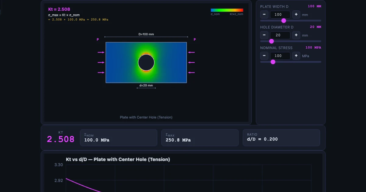
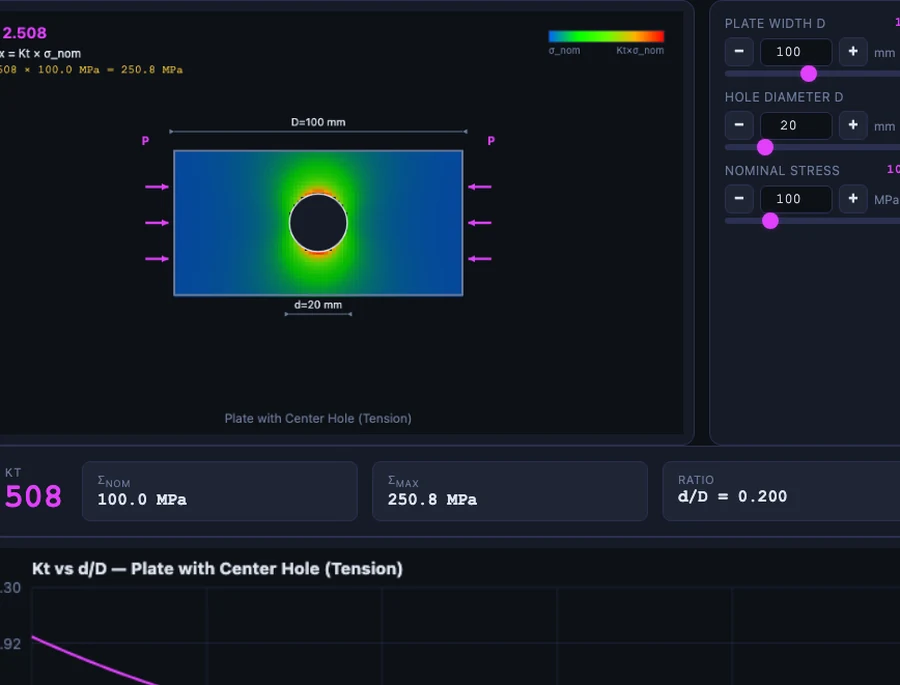
For each geometry, the simulator uses the Peterson polynomial formula for that specific case, evaluated in real time as you move the sliders. The geometry sketch updates as you adjust the parameters so you always know what you’re calculating. The colour stress map shows qualitatively where the concentration is highest. And the K_t value sits in a large readout at the top — because that single number is what you need for every downstream calculation.

I’ll use the two most pedagogically important cases as worked examples: the plate with a central hole, and the shaft with a shoulder fillet under bending.

The Classic Case: Plate With a Central Hole

The plate with a central hole under uniaxial tension is the textbook introduction to stress concentration for good reason: it has an exact analytical solution in the limit of an infinite plate (due to Kirsch, 1898), and the result is memorable. As the hole diameter shrinks relative to the plate width — as d/W approaches zero — K_t approaches exactly 3.0. Three times the nominal stress, right at the edge of the hole, oriented perpendicular to the loading direction.

\[K_t \to 3.0 \quad \text{as } d/W \to 0\]

This is the infinite-plate result, independent of hole size, material, and load. It holds as long as the stress state is elastic and the plate is wide relative to the hole. The practical Peterson polynomial for a finite plate with a central hole is:

\[K_t = 3 - 3.13\!\left(\tfrac{2r}{W}\right) + 3.66\!\left(\tfrac{2r}{W}\right)^{\!2} - 1.53\!\left(\tfrac{2r}{W}\right)^{\!3}\]

where r is the hole radius and W is the total plate width. At d/W = 0 (or equivalently 2r/W = 0), this collapses to K_t = 3.0 exactly. As the hole grows larger relative to the plate width, K_t actually decreases — because the net section area is shrinking, and the nominal stress on that reduced section is rising to meet the local stress. The worst design from a concentration standpoint is a small, sharp hole in an otherwise wide plate, not a large one.

The colour stress map in the simulator makes this tangible. At d/W = 0.1, the red concentration zones at the top and bottom of the hole are narrow and intense. As you drag d/W toward 0.5, the red zones spread and soften — the concentration factor is falling, but the plate is getting seriously weakened. Neither extreme is a good design; the stress concentration factor and the net-section stress are in tension with each other, and both must be checked.

I use this geometry to introduce the concept of “stress flow lines” — imaginary trajectories that carry the load through the cross-section. Around a hole, those lines have to detour, and wherever they crowd together, the stress is high. Once students visualise that analogy, they can predict qualitatively where the concentration will be on any geometry before running any numbers.

Shaft Fillets: Where Real Failures Start

If the plate-with-hole case is the classroom introduction, the shaft shoulder fillet is the engineering reality. The vast majority of fatigue failures in rotating machinery — shafts, axles, crankshafts, camshafts — initiate at cross-section changes. A step-down in diameter is unavoidable in practical shaft design: you need a larger diameter to support a bearing, a smaller one to fit a coupling or gear, and a transition between them. That transition is the fillet, and its radius determines K_t.

For a shaft under bending with a shoulder fillet, K_t is a function of two dimensionless ratios: r/d (fillet radius over smaller shaft diameter) and D/d (larger diameter over smaller diameter). At r/d = 0.1 and D/d = 1.5, Peterson’s formula gives K_t ≈ 2.05. That’s the operating point shown in the body image above. Now drag the fillet radius toward zero:

• r/d = 0.1 → K_t ≈ 2.05
• r/d = 0.05 → K_t ≈ 2.7
• r/d = 0.02 → K_t > 3.5

A 1 mm fillet on a 20 mm shaft (r/d = 0.05) nearly doubles the stress concentration compared to a modest 2 mm fillet (r/d = 0.1). The engineering effort to go from 1 mm to 2 mm at the tool-path level is negligible. The difference in component life is not.

What the Kt vs r/d curve in the simulator shows so clearly is the asymptotic behaviour. Below r/d ≈ 0.05, K_t climbs steeply — small changes in fillet radius produce large changes in stress. Above r/d ≈ 0.2, the curve flattens and further increases in fillet radius give diminishing returns. The designer’s target zone is typically 0.1 to 0.2 for shafts under fatigue loading. Engineers who know this never again specify a sharp corner on a rotating shaft. The ones who don’t know it keep getting surprised by failures.

The shaft torsion case (geometry 6) follows a similar pattern, with K_t values that are generally lower than the bending case for the same r/d. The bending case is more critical because the outer fibre of the shaft — where bending stress is maximum — coincides with the fillet location. For combined bending and torsion, you’ll want the Shaft Torsion Simulator to resolve the individual stress components before applying K_t.

From Kt to Fatigue: The Kf Connection

K_t is a geometric, elastic quantity. In fatigue design, we need K_f — the fatigue stress concentration factor — which accounts for the material’s actual sensitivity to notches. The relationship is:

\[K_f = 1 + q(K_t - 1)\]

where q is the notch sensitivity index, ranging from 0 (completely insensitive) to 1 (fully sensitive, K_f = K_t). Notch sensitivity depends on material strength and notch radius; it’s tabulated in Peterson’s charts and in Shigley’s Appendix tables.

For Steel 4140 with S_ut = 1020 MPa at a notch radius of 1 mm, q ≈ 0.92. Applying the shaft fillet bending case at r/d = 0.1, D/d = 1.5 (K_t ≈ 2.05):

\[K_f = 1 + q(K_t - 1) = 1 + 0.92 \times (2.05 - 1) = 1 + 0.966 = 1.97\]

So the effective fatigue stress concentration factor is 1.97. In the Marin equation for fatigue, this becomes k_e = 1/K_f = 1/1.97 ≈ 0.51. The corrected endurance limit is just over half the laboratory value. That single number — derived from a 1 mm fillet on a 20 mm shaft — can cut the predicted fatigue life by more than a factor of two compared to ignoring the notch entirely.

High-strength steels like 4140 have high notch sensitivity (q near 1), which means K_f ≈ K_t. Mild steels have q around 0.6–0.7, so K_f is meaningfully lower than K_t. Cast iron is nearly notch-insensitive (q near 0) because its internal graphite flakes already act as stress raisers, pre-empting the external geometry. This is why high-strength steel is not always the right material choice for notch-critical fatigue applications — a lower-strength steel with lower notch sensitivity can outperform it at a stress-concentrated location.

For the full fatigue analysis workflow, the fatigue life simulator teaching guide covers the Marin correction factors, the Goodman diagram, and how to integrate K_f into a complete endurance limit calculation.

How I Use This in My Stress Analysis Unit

I run the stress concentration topic over two sessions at the start of the Stress Analysis unit. Here’s the flow that’s worked best.

Session 1: Discovery before formulas. I don’t open a textbook. I put the simulator on the projector, select the plate-with-central-hole geometry, and ask students to predict what happens to the stress at the hole edge as the hole gets smaller. Most guess it goes down — smaller hole, less disruption. I move the slider and show them K_t climbing toward 3.0. The room goes quiet. Then I explain the stress-flow-lines mental model, show the colour map, and only then introduce the formula and its derivation. The formula lands as an explanation of something they’ve already seen, not as an abstract equation to memorise.

Session 2: Shaft fillet design exercise. Students get a design brief: a 20 mm step-down shaft in Steel 4140, D/d = 1.5, rotating bending load, 10⁷ cycle design life. Their job is to choose a fillet radius that keeps K_f below 2.0. They use the simulator to find K_t at different r/d values, look up q for 4140 at the fillet radius, compute K_f, and iterate. When they find that r/d ≈ 0.1 (a 1 mm fillet) sits right on the K_f = 2.0 boundary, and that going to 1.5 mm drops it to 1.85, they’ve just done real engineering design. The simulator turns what would have been a chart-lookup exercise into a design iteration exercise.

I finish the second session by linking back to the fatigue unit: I ask students to open the Fatigue Life Simulator, enter K_f = 1.97 as k_e = 0.51, and see what it does to the corrected endurance limit for their 4140 shaft. Watching S_e drop from 510 MPa to around 230 MPa in one input field change is more persuasive than any lecture I could give. They write the number down. They’re not forgetting it.