Heat Transfer — Conduction, Convection and Radiation Explained with a Simulator

Ask an engineering student to name the three modes of heat transfer and they will answer without hesitation: conduction, convection, radiation. Ask them to explain why a metal rod conducts heat faster than a brick, or why doubling the wall thickness halves the heat loss rather than halving it proportionally in a non-linear way, and the answer is less certain. The names are easy. The physics behind each mode — and especially the formulas that quantify them — are where the difficulty lives.

A free browser-based heat transfer simulator puts all three modes in one tool. Switch between Conduction, Convection, and Radiation with a single button. Adjust material, thickness, temperature, surface area, or emissivity and watch the heat transfer rate and thermal resistance update in real time. The formula is displayed on screen and the answer recalculates instantly — so students can see exactly how each variable drives the result before writing anything on paper.

Why Heat Transfer Feels Abstract in a Classroom

Conduction, convection, and radiation are invisible. You can hold a hot mug and feel the conduction through the ceramic, but you can’t see the molecular vibrations carrying energy from the inner wall to the outer surface. You can feel warm air rising from a radiator, but the boundary-layer physics that governs Newton’s Law of Cooling is not visible. Radiation from the sun is felt as warmth but carries no material at all.

This is the core teaching challenge. Unlike beam bending where you can see a deflection, or a hydraulic circuit where oil visibly flows, heat transfer happens at a scale that is difficult to point at. A simulator that animates the energy flow — particles moving through a wall gradient, fluid sweeping over a hot surface, radiation arrows leaving a glowing body — gives the invisible a visible proxy. That proxy is what turns a formula into an intuition.

Mode 1: Conduction and Fourier’s Law

Conduction is heat transfer through a solid material. The atoms don’t move — they vibrate in place and pass energy to their neighbours through molecular collisions. Metals conduct heat rapidly because their free electrons carry energy efficiently. Bricks and polymers conduct slowly because their atomic bonds transfer energy reluctantly.

The governing equation is Fourier’s Law:

Q = k × A × ΔT / L

Where Q is the heat transfer rate (watts), k is the thermal conductivity of the material (W/m·K), A is the cross-sectional area (m²), ΔT is the temperature difference across the wall (K), and L is the wall thickness (m).

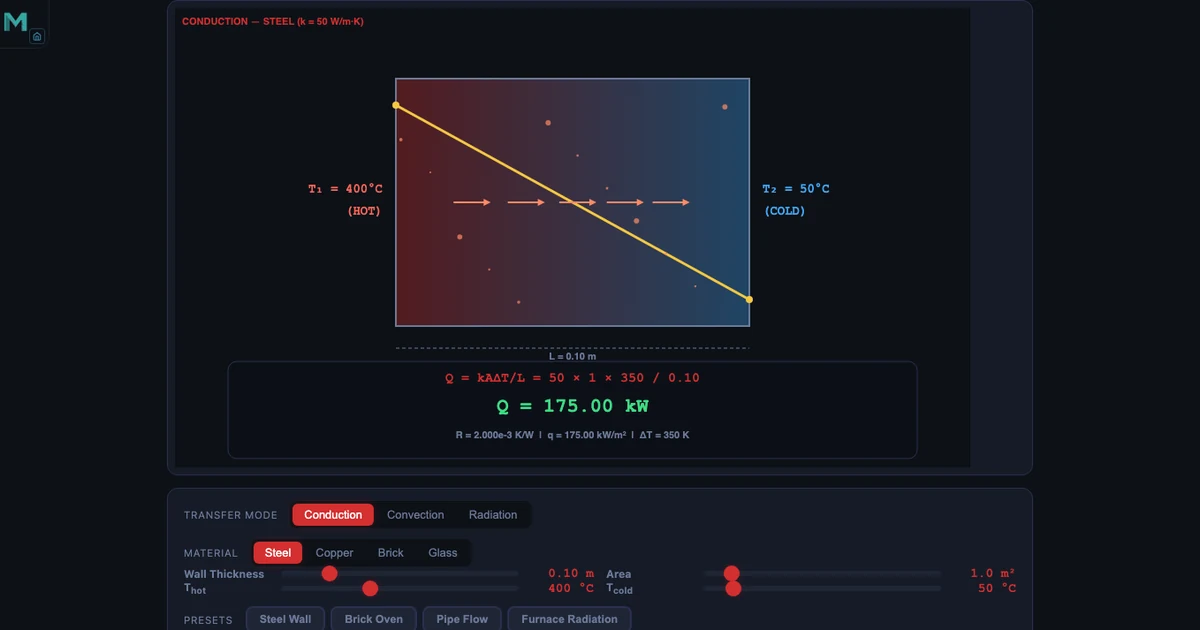
The simulator hero image above shows a steel wall (k = 50 W/m·K) with T_hot = 400 °C and T_cold = 50 °C across 0.10 m of thickness, 1.0 m² of area. The formula resolves live on screen:

Q = 50 × 1 × 350 / 0.10 = 175.00 kW

Switch the material from Steel (k = 50) to Copper (k = 385) and the heat rate jumps immediately — copper conducts nearly eight times more heat for the same geometry. Switch to Brick (k ≈ 0.7) and the rate drops to a fraction of the steel value. The same ΔT, the same wall dimensions, radically different heat flows. That comparison delivers more intuition about thermal conductivity than a table of values ever will.

Thermal resistance is the analogue of electrical resistance and it makes multi-layer wall problems tractable:

R_cond = L / (k × A)   →   Q = ΔT / R

For the steel wall: R = 0.10 / (50 × 1) = 0.0020 K/W — exactly the readout on the simulator. For composite walls, R_total = R₁ + R₂ + R₃, just like resistors in series. This is the tool that makes building insulation analysis tractable by hand.

Mode 2: Convection and Newton’s Law of Cooling

Convection transfers heat between a solid surface and a moving fluid. The fluid carries warm particles away from the surface and replaces them with cooler ones — a continuous process that depends on how fast the fluid moves and how it interacts with the surface boundary layer.

Newton’s Law of Cooling:

Q = h × A × (T_surface − T_fluid)

Where h is the convective heat transfer coefficient (W/m²·K). The value of h is where the complexity lives. Natural convection in still air: h ≈ 5–25 W/m²·K. Forced convection with a fan: h ≈ 25–250. Liquid water flowing over a surface: h ≈ 500–10,000. These ranges span three orders of magnitude and explain why water-cooled systems transfer heat so much more effectively than air-cooled ones.

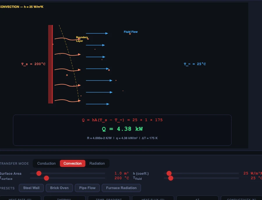
The simulator’s Convection mode shows this numerically. At the default h = 25 W/m²·K with T_surface = 200 °C and T_fluid = 25 °C over 1.0 m²:

Q = 25 × 1 × (200 − 25) = 25 × 175 = 4.38 kW

Increase h to 250 (forced convection) and Q jumps to 43.8 kW — ten times the heat transfer from the same surface under the same temperature difference. That is the engineering argument for a cooling fan.

Mode 3: Radiation and the Stefan-Boltzmann Law

Radiation requires no medium. It is heat transfer by electromagnetic waves — the same process that carries energy from the sun across 150 million kilometres of vacuum to warm the Earth’s surface. Every object above absolute zero emits radiation. The Stefan-Boltzmann Law gives the rate:

Q_rad = ε × σ × A × T⁴

Where ε is the emissivity (0–1), σ = 5.67 × 10⁻⁸ W/m²·K⁴ (Stefan-Boltzmann constant), and T is the absolute temperature in kelvin. Notice the T⁴ dependence. Double the absolute temperature and the radiation rate increases by a factor of sixteen. This is why radiation dominates heat transfer in high-temperature applications — furnaces, gas turbines, re-entry vehicles — and is often negligible at room temperature.

Emissivity is a material surface property. Polished aluminium: ε ≈ 0.05 (reflects most radiation). Black paint or oxidised steel: ε ≈ 0.9–0.95 (emits nearly as much as a perfect blackbody). A solar-thermal collector is coated to maximise absorptivity (same physics as emissivity, by Kirchhoff’s law). An industrial furnace lining is selected for high emissivity to maximise heat delivery to the workpiece.

The Radiation mode in the simulator lets students slide emissivity from 0.05 to 1.0 and temperature from low to high, watching the T⁴ effect play out quantitatively. It is one of the fastest ways to internalise why T⁴ is in the formula rather than T or T².

Thermal Resistance — The Unifying Framework

The most useful concept in an applied heat transfer course is thermal resistance, because it makes every mode algebraically comparable and allows composite systems to be solved with simple addition.

• Conduction resistance: R_cond = L / (k × A)
• Convection resistance: R_conv = 1 / (h × A)
• Total Q through a series system: Q = ΔT_total / R_total

Consider a brick wall with convection on both sides. Five resistances in series: R_conv,hot + R_brick + R_conv,cold. Add them, divide the overall temperature difference, and you have the steady-state heat flux through the entire assembly. This is the calculation behind every building energy rating, every heat exchanger design, and every thermal management system in electronics.

The simulator calculates and displays R for whatever mode is active. Students can verify that R_cond = 0.0020 K/W for the 0.10 m steel wall, check it equals L/(k×A) = 0.10/(50×1), and then understand why switching to Brick (k = 0.7) makes R jump to 0.143 K/W — 70 times higher, 70 times less heat transferred.

How to Use the Simulator in Class

Start with a material comparison on Conduction mode. Set identical geometry: L = 0.10 m, A = 1.0 m², T_hot = 400 °C, T_cold = 50 °C. Cycle through Steel, Copper, Brick, and Glass. Ask the class to predict the ordering before clicking. Steel conducts well (k = 50); Copper much better (k = 385); Brick very poorly (k ≈ 0.7). When they see the numbers confirm their prediction, the material-property table starts making sense.

Demonstrate the thickness effect. Hold everything fixed on Steel and slide the Wall Thickness from 0.10 m to 0.20 m. Q halves. To 0.05 m: Q doubles. Students who see this direct linear relationship between thickness and resistance — R = L/kA — rarely forget it.

Show why convection coefficient matters more than surface temperature. On Convection mode, set T_surface = 300 °C, T_fluid = 25 °C, h = 25. Note Q. Now reduce T_surface to 200 °C but increase h to 250 (simulating a fan). Q increases despite a lower surface temperature, because h dominates. This is the design insight behind forced-air cooling in electronics.

Use the presets for scenario-based learning. The four presets (Steel Wall, Brick Oven, Pipe Flow, Furnace Radiation) represent real engineering scenarios. Load “Brick Oven” and discuss the thermal resistance of a kiln wall. Load “Furnace Radiation” and discuss why radiation becomes the dominant mode at furnace temperatures. Each preset is a conversation starter that connects the formula to an application students have seen.

For the engine thermodynamics context where combustion heat is converted to mechanical work, see our article on the four-stroke engine cycle and PV diagram — heat transfer is the input to every thermodynamic cycle.