Heat Transfer Modes Explained: Conduction, Convection and Radiation with a Free Simulator
Heat transfer sits at the core of almost every engineering system you can name. Engines reject waste heat. Buildings lose energy through walls. Electronics fail when they overheat. Rocket nozzles survive temperatures that would vaporise most metals. Understanding how heat moves — and more specifically, which of the three modes dominates in a given situation — is not optional knowledge. It's the difference between a design that works and one that burns up on the first run.
The MechSimulator Heat Transfer tool covers all three modes — conduction, convection, and radiation — in a single interface with four realistic presets and a full Explore library of 12 concepts. This article walks through each mode using the simulator's real output numbers.
Why Students Mix Up the Three Modes
The confusion usually starts with the mental model. Students picture heat as a fluid that "flows through" things — fine for conduction, misleading for radiation. Conduction needs physical contact. Convection needs a moving fluid. Radiation needs nothing at all; it works perfectly well across a vacuum, which is exactly how the Sun's energy reaches Earth.
Here is the real problem: the three modes use different governing equations with different parameter sets. Conduction uses thermal conductivity k (a material property). Convection uses a heat transfer coefficient h (depends on geometry and flow conditions). Radiation uses emissivity ε and temperature raised to the fourth power. These are not interchangeable. You cannot substitute the wrong equation and expect a sensible answer.
The simulator forces the issue. Switching between the three mode tabs shows that each has its own controls, its own formula card, and its own output. After spending five minutes switching between conduction and radiation, students stop conflating them.
Mode 1 — Conduction: Fourier's Law
Fourier's Law quantifies heat transfer through a solid by a temperature gradient driving heat flux across a cross-section:
\[Q = \dfrac{kA(T_1 - T_2)}{L}\]
where \(k\) is thermal conductivity (W/m·K), \(A\) is the cross-sectional area (m²), and \(L\) is the wall thickness (m). Thermal conductivity spans a remarkable range: copper k ≈ 385 W/m·K; steel k ≈ 50 W/m·K; brick k ≈ 0.7 W/m·K; aerogel insulation k ≈ 0.015 W/m·K. A brick wall is 3,300 times worse at conducting heat than steel.
The thermal resistance analogy is worth dwelling on. Define:
\[R_{\text{th}} = \dfrac{L}{kA} \quad \text{(K/W)}\]
Then Q = ΔT / R_th — identical in form to Ohm's Law V = I·R. For a composite wall (several materials in series), you simply add the resistances: R_total = R₁ + R₂ + ···. This is the key insight that makes building envelope calculations tractable.
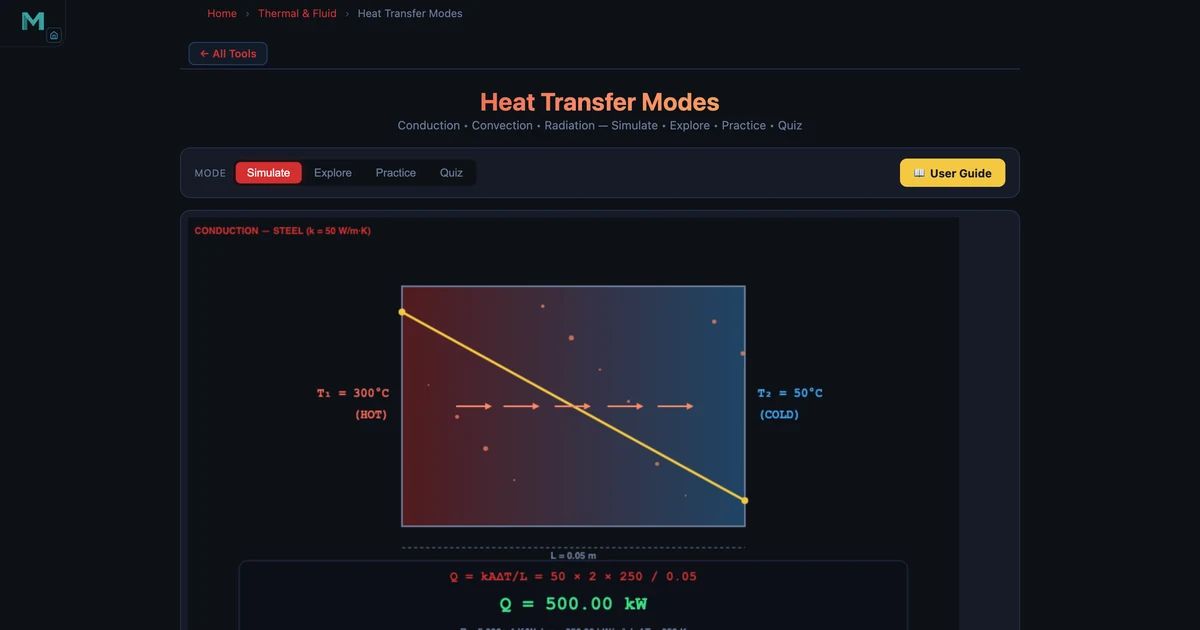
Steel Wall preset (hero image above): k = 50 W/m·K, L = 0.05 m, A = 2 m², T₁ = 300 °C, T₂ = 50 °C. The simulator confirms:
\[Q = \dfrac{50 \times 2 \times 250}{0.05} = 500{,}000 \text{ W} = 500 \text{ kW}\]
\[R_{\text{th}} = \dfrac{0.05}{50 \times 2} = 5.00 \times 10^{-4} \text{ K/W}\]
The temperature gradient across the wall is 5000 K/m — 5 °C per millimetre. Heat flux (power per unit area) is 250 kW/m². These are the numbers visible in the readout cards in the hero image.
The Brick Oven preset (k = 0.7 W/m·K, L = 0.2 m) shows how dramatically lower conductivity reduces the heat flow even with a much larger temperature difference. That comparison — steel vs brick, same ΔT — is what solidifies the meaning of k as a material property.
Mode 2 — Convection: Newton's Law of Cooling
Convection transfers heat between a solid surface and an adjacent fluid by combined conduction through the fluid and bulk fluid motion. Newton's law of cooling:
\[Q = hA(T_s - T_\infty)\]
where h is the convection coefficient (W/m²·K), T_s is the surface temperature, and \(T_\infty\) is the undisturbed fluid temperature. The h value encodes everything about the fluid's physical properties and the flow geometry:
- Natural convection (air): h ≈ 5–25 W/m²·K — buoyancy-driven, slow.
- Forced convection (air fan): h ≈ 25–250 W/m²·K — mechanically assisted, faster.
- Forced convection (water): h ≈ 100–1000 W/m²·K — water's high density gives it much better heat removal.
- Boiling water: h ≈ 2500–25000 W/m²·K — phase change enormously increases the effective coefficient.
The Pipe Flow preset — A = 2 m², h = 150 W/m²·K, T_s = 120 °C, T_fluid = 30 °C — loads a forced-convection scenario. The simulator computes Q = hA(T_s − T∞) = 150 × 2 × 90 = 27,000 W = 27 kW. Adjust the h slider from 150 to 500 and watch Q jump from 27 kW to 90 kW with the same geometry. That's the payoff for adding a pump to a cooling loop.
Mode 3 — Radiation: Stefan-Boltzmann Law
Radiation is the odd one out. No contact, no medium, no moving fluid — just electromagnetic energy emitted by any body with a temperature above absolute zero. The net heat exchanged between a surface and its surroundings:
\[Q = \varepsilon \sigma A (T_1^4 - T_2^4)\]
where \(\varepsilon\) is emissivity (0 to 1), \(\sigma = 5.67 \times 10^{-8}\) W/(m²·K⁴) is the Stefan-Boltzmann constant, and temperatures are in Kelvin — mandatory, not optional. A common exam error is substituting Celsius; the T⁴ term makes the result wildly wrong.
The T⁴ dependence is the reason furnaces and industrial kilns are dominated by radiation while a room-temperature desktop computer is not. Double the absolute temperature and the radiated power increases by 2⁴ = 16 times.

Furnace Radiation preset: ε = 0.9, A = 2 m², T₁ = 1000 K, T₂ = 300 K. The simulator reports Q = 101.23 kW. Let's verify:
\[Q = 0.9 \times 5.67\times10^{-8} \times 2 \times (1000^4 - 300^4)\]
\[= 0.9 \times 5.67\times10^{-8} \times 2 \times (1.0\times10^{12} - 8.1\times10^{9}) = 101{,}230 \text{ W} \approx 101.2 \text{ kW}\]
A polished metal surface has ε ≈ 0.05 — it emits and absorbs only 5% of what a blackbody would. An oxidised steel surface has ε ≈ 0.8. That's why thermos flasks have silvered inner walls: minimising emissivity reduces radiant heat exchange dramatically.
Comparing the Three Modes
No single mode dominates in all conditions. A rough guide:
- Below 200 °C: Conduction and convection typically dominate. Use Fourier's Law and Newton's Cooling.
- 200–600 °C: All three modes contribute significantly. Radiation begins to compete with convection.
- Above 600 °C: Radiation usually carries the majority of the heat. The T⁴ scaling overwhelms conduction and convection.
The Explore mode in the simulator documents this with four concept categories: conduction, convection, radiation, and worked examples. Twelve concepts total — Fourier's Law, thermal resistance, composite wall, Newton's Cooling, natural vs forced convection, Stefan-Boltzmann Law, emissivity, blackbody radiation, and more. Each card shows the formula, a physical description, and a numeric worked example.
How to Use This in a Lesson
Opening question (3 min). Ask: how does heat from the Sun reach Earth? No atmosphere at the source, no medium between, yet 1361 W/m² arrives. Students who reflexively say "conduction" pause. Radiation — electromagnetic waves — is the only mode that works in vacuum.
Conduction demo (8 min). Load the Steel Wall preset and record Q. Then switch to Brick with the same ΔT and record again. Divide. The ratio of Q values equals the ratio of k values. Students have just empirically confirmed that thermal conductivity scales the heat flow linearly — no equation needed to see it.
Convection slider experiment (5 min). In Pipe Flow, drag the h slider from 10 (natural convection) to 200 (forced). Ask students to describe the engineering change that each slider position represents — a fan, a pump, a wind gust, boiling. This maps numbers to physical situations.
Radiation temperature sensitivity (5 min). In the Radiation mode, start at T₁ = 400 K and record Q. Then increase T₁ to 800 K — double the temperature. Ask students to predict Q. It will be 2⁴ = 16 times larger. This demonstration makes the T⁴ relationship memorable in a way that writing the exponent never does. For context on why gas temperature matters in enclosed systems, the Ideal Gas Law guide explains how temperature drives pressure in closed volumes — a related thermal concept.
Practice and Quiz (7 min). The Practice mode generates randomised heat transfer problems (conduction, convection, and radiation) with full step-by-step solutions shown after each attempt. The Quiz mode delivers five scored questions per session — a complete formative assessment built in.
Try It Yourself
All tools below are free — no account, no download.
Key Takeaways
- Conduction requires direct contact. Q = kAΔT/L. Thermal conductivity k ranges from 0.015 W/m·K (aerogel) to 385 W/m·K (copper).
- Thermal resistance R_th = L/(kA) is exactly analogous to electrical resistance — composite walls add resistances in series.
- Convection requires fluid motion. Q = hA(T_s − T∞). Forced convection gives h ≈ 25–500 W/m²·K; natural convection gives 5–25 W/m²·K.
- Radiation requires no medium. Q = εσA(T₁⁴ − T₂⁴). Temperatures must be in Kelvin. At 1000 K, a surface with ε = 0.9 delivers 101.23 kW.
- The T⁴ dependence of radiation means doubling absolute temperature increases radiated power by 16×. Above ~600 °C, radiation typically dominates.
- The simulator's Explore mode documents 12 concepts across all three modes with worked examples and numeric answers — a complete reference for exam preparation.
Frequently Asked Questions
What is Fourier's Law of heat conduction?
Fourier's Law states that the rate of heat transfer through a solid is Q = kA(T₁ − T₂)/L, where k is thermal conductivity (W/m·K), A is cross-sectional area (m²), ΔT is temperature difference (K), and L is thickness (m). For a steel wall (k = 50 W/m·K) 0.05 m thick, 2 m² area, ΔT = 250 K, the simulator confirms Q = 500 kW.
What is Newton's Law of Cooling?
Newton's Law of Cooling describes convective heat transfer: Q = hA(T_s − T∞), where h is the convection coefficient (W/m²·K), A is surface area, T_s is surface temperature, and T∞ is the ambient fluid temperature. Natural convection gives h ≈ 5–25 W/m²·K; forced convection gives h ≈ 25–500 W/m²·K.
How does radiation heat transfer differ from conduction and convection?
Radiation transfers heat by electromagnetic waves and requires no medium — it works in a vacuum. Its governing equation is Q = εσA(T₁⁴ − T₂⁴), where ε is emissivity and σ = 5.67×10⁻⁸ W/(m²·K⁴). The T⁴ dependence makes radiation dominant at high temperatures. At 1000 K, a surface with ε = 0.9 radiates 101.23 kW — more than conduction through most walls.
What is thermal resistance and how is it like electrical resistance?
Thermal resistance R = L/(kA) for conduction (K/W) is analogous to electrical resistance R = L/(σA) for current flow. Just as V = IR gives voltage from current and resistance, ΔT = Q·R gives temperature difference from heat flow and thermal resistance. For layers in series (composite wall), thermal resistances add: R_total = R₁ + R₂ + ...
Which heat transfer mode dominates at high temperatures?
Radiation dominates at high temperatures because it scales with T⁴. At low temperatures (below ~300 K) conduction and convection dominate. Above ~800 K, radiation often carries more energy than both combined. The Furnace Radiation preset in the simulator — ε = 0.9, T₁ = 1000 K, T₂ = 300 K — delivers Q = 101.23 kW, demonstrating radiation's power at furnace temperatures.
Heat transfer is one of those subjects where knowing the three equations is necessary but not sufficient. You also need an intuition for which mode dominates in a given situation — and that only comes from working with the numbers across different scenarios.
Load the Heat Transfer Simulator, switch between presets, and try doubling T₁ in the radiation mode. The jump in Q is the moment the T⁴ rule becomes physical rather than algebraic.