Steam Engine Simulator
Reciprocating Engine Lab — Slide Valve • Indicator Diagram • Compound • 2D & 3D


Display Controls
The crank is barred off dead centre. Open the stop valve: steam reaches the chest and the engine accelerates against a dynamo whose torque rises with speed; the flywheel carries it through the dead centres. With the governor on, the cut-off shortens as the speed rises above the set speed (6 % droop); switch it off and the speed wanders with the load. Every reading is the full cycle solved at the present speed and cut-off, in real time.
⚙ Valve gear, steam, friction & flywheel
The slide valve is driven by a single eccentric through a rocker; its steam lap is solved so that the cover end cuts off at the set fraction, with the travel, lead and exhaust lap you choose. Expansion and compression follow pVn = C. Release and admission take a few degrees of crank as the port opens. Steam consumption counts the charge at cut-off less the cushion steam kept at compression, plus the missing quantity.
Σ Live equations — values substituted from the current engine
📋 Valve events — admission, cut-off, release and compression for each end
⚡ Efficiency ladder — Carnot, Rankine, modified Rankine and the engine
💡 What-if coach — insights from the current engine
1 Overview
The Steam Engine Simulator runs a horizontal, double-acting reciprocating steam engine with a D slide valve. Choose a simple engine exhausting to the atmosphere, a condensing engine exhausting to a vacuum, or a tandem compound with high- and low-pressure cylinders on one piston rod. The valve events come from the valve gear itself, and every number on the page — the colours in the section, the four diagrams, the readouts, the 3D engine and the step-by-step calculations — comes from the one solved engine.
Four modes: Simulate, Explore (20 illustrated concept cards with worked examples), Practice (12 types of generated problems with full solutions) and Quiz (6 questions drawn from a pool of 22).
2 Choosing the engine and the view
The strip above the canvas picks the Engine — Simple, Condensing or Compound — and the View, 2D or 3D. A computer or tablet opens in 3D and a phone in 2D; your own choice is remembered. The Preset list offers engines of that kind: a textbook engine, a traction engine cylinder, a locomotive cylinder notched up, a school model, a condensing mill engine, a launch engine and two compounds. Presets are representative classes of engine, not the data of a particular machine.
3 Simulate mode — the 2D section and diagrams
The left of the canvas is the engine cut on its centre line: steam chest, slide valve and ports above the cylinder; the piston, piston rod, crosshead in its guides, connecting rod, crank, eccentric, rocker and flywheel. Each end of the cylinder is coloured by its steam pressure, from blue exhaust to white-hot live steam, and arrows show steam flowing through any open port. The line under the cylinder marks cut-off, release and compression for both ends. The text at the top names the phase each end is in.
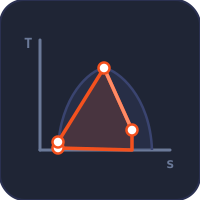
The right pane shows one of four diagrams: p–V (the indicator diagram of both ends, with the hypothetical diagram dotted; a compound shows both cylinders as a combined diagram), Valve (the Zeuner diagram with lap circles, port openings and the four events), Torque (the crank-effort diagram, its mean and the flywheel’s fluctuation of energy) and T–s (the modified Rankine cycle on the steam dome).
Pause freezes the engine; +10° turns it ten degrees; or drag the flywheel to turn it by hand. Display Controls (top-left of the canvas) switch the colours, puffs, event marks, labels, grid and hypothetical diagram.
4 The 3D engine
In 3D the same engine stands on its bed: cylinder with its lagging and steam chest, the slide valve inside, piston and rods, crosshead and guide bars, connecting rod, crank, main bearings, eccentric and rocker, flywheel, exhaust pipe and governor. Drag to turn it, pinch or Ctrl + scroll to zoom, and click any part for a card that says what it does and gives its live numbers. Cutaway opens the cylinder and steam chest on their centre line, X-ray makes the casings glass and Exterior shows the engine closed. The steam inside each end glows at the colour of its pressure.
5 Run engine — stop valve, load and governor
Run engine opens a panel. Open stop valve lets steam into the chest; the engine accelerates against a dynamo load whose torque rises with speed, and the flywheel carries it through the dead centres. The Load slider sets the brake load as a percentage of the rated torque. With the Governor on, the cut-off shortens as the speed rises above the set speed (a proportional governor with 6 % droop); with it off the cut-off stays where you set it and the speed settles wherever the load allows. Close stop valve lets it run down. Sound is a chuff at each exhaust beat, synthesised in your browser and started only by a button.
6 Controls and what they change
Steam-chest pressure p1 and back pressure pb (both absolute), cut-off (cover end, as a fraction of the stroke), speed, bore and stroke; the compound adds the LP bore and LP cut-off. The advanced panel holds the piston-rod diameter, the connecting-rod ratio, the clearance volume, the valve travel, lead and exhaust lap, the dryness fraction, the expansion index, the mechanical efficiency, the missing quantity, the reciprocating mass and the flywheel. In a compound the two valves share one spindle, so the LP valve has the same travel and angle of advance as the HP and its lead follows from its lap.
7 Reading the results
Indicated power IP from the indicator diagrams, brake power BP = ηm·IP and the brake torque; the mean effective pressure of each end and the diagram factor; steam consumption and specific steam consumption; the indicated thermal efficiency against the Rankine and modified Rankine efficiencies; the release pressure (or the receiver pressure of a compound); and the speed fluctuation the flywheel allows. The calculator button opens every step. Export saves the indicator diagrams and crank torque as CSV or the canvas as PNG.
8 Explore, Practice and Quiz
Explore has five categories: How It Works, Indicator Diagram, Slide Valve, Performance, and Crank & Flywheel; every worked number in a card is computed by the same engine. Practice generates a new problem each time (hypothetical and actual mean effective pressure, indicated and brake power, torque, angle of advance, the crank angle at cut-off, piston position with a finite connecting rod, specific steam consumption, thermal efficiency, flywheel speed fluctuation and piston force); type your answer, check it, or reveal the worked solution. Quiz asks six questions with shuffled options and scores you with stars.
9 SI and Imperial units
SI shows bar, mm, kW, kg/h, kg/kWh, kN·m and °C. Imperial shows psia, inches, horsepower, lb/h, lb/(hp·h), lbf·ft and °F; piston speed is in ft/min. For example 8 bar is 116.0 psia and 22.4 kg/kWh is 36.8 lb/(hp·h). The canvas, the diagrams, the tables and the CSV follow the switch; the live equations, the calculation modal, the Explore examples and the Practice problems are worked in SI, as the textbooks are. Your choice is remembered across the site.
10 Tips
Start with the Textbook simple engine and shorten the cut-off: the indicator diagram gets thinner, the power falls and the steam per kWh falls too. Switch to Condensing and watch the back-pressure line drop below the atmosphere. Lower the connecting-rod ratio to 3 and compare the cut-off of the two ends. Raise the exhaust lap until the compression curve climbs past the steam-chest pressure and forms a loop. In Run engine, switch the governor off and change the load.
Steam Engine Simulator: How a Reciprocating Steam Engine Works
A reciprocating steam engine turns the pressure of steam into work on a piston. Steam from the boiler fills the steam chest; a slide valve moving over three ports lets it into one end of the cylinder while it connects the other end to the exhaust. The steam pushes the piston, the piston rod and crosshead carry the push to the connecting rod, and the rod turns the crank. The valve shuts off the steam part-way along the stroke — the cut-off — and the trapped steam keeps pushing as it expands. A flywheel carries the crank through the two dead centres. This free steam engine simulator runs that machine in a 2D section and in 3D, and draws the indicator diagram, the valve diagram, the crank effort and the cycle as it turns.
The Six Events of Each Stroke
Each end of a double-acting cylinder goes through the same sequence once a revolution: admission (the port opens just before dead centre, the lead), cut-off, expansion, release (the port opens to the exhaust near the end of the stroke), exhaust on the return stroke and compression (the exhaust closes and the remaining steam is squeezed into the clearance as a cushion). The two ends are half a revolution apart, so while one is admitting the other is exhausting.
The Steam Engine Indicator Diagram and Mean Effective Pressure
An indicator diagram plots the pressure in the cylinder against the piston’s position. Its area is the work done on the piston in one stroke, and dividing that work by the swept volume gives the mean effective pressure, pm. For the textbook hypothetical indicator diagram — admission at constant pressure p1, hyperbolic expansion pV = C to the end of the stroke, an instant drop and exhaust at the back pressure pb, with clearance and compression neglected —
pm = (p1/r)(1 + ln r) − pb, r = 1 / cut-off
The real card has rounded corners, and the diagram factor k is the ratio of the real area to the hypothetical one. The table is the simulator’s textbook engine (300 × 450 mm, 8 bar, exhausting at 1.1 bar, 150 rpm) at different cut-offs:
| Cut-off | Expansion ratio r | Hypothetical pm (bar) | Simulated pm, cover end (bar) | Indicated power (kW) | Steam (kg/kWh) | Indicated η |
|---|---|---|---|---|---|---|
| 20 % | 5.00 | 3.08 | 2.80 | 40.2 | 16.9 | 11.0 % |
| 25 % | 4.00 | 3.67 | 3.32 | 47.9 | 17.8 | 10.4 % |
| 33 % | 3.00 | 4.50 | 4.08 | 59.4 | 19.3 | 9.6 % |
| 40 % | 2.50 | 5.03 | 4.59 | 67.4 | 20.5 | 9.0 % |
| 50 % | 2.00 | 5.67 | 5.24 | 78.0 | 22.4 | 8.3 % |
| 60 % | 1.67 | 6.15 | 5.76 | 87.0 | 24.4 | 7.6 % |
| 75 % | 1.33 | 6.63 | 6.36 | 97.8 | 27.8 | 6.7 % |
Cutting off earlier gives less power but more work from each kilogram of steam. The simulated diagram has no wire-drawing through the ports, so its diagram factor (about 0.9 here) is at the top of the 0.6–0.9 found on real engines.
Indicated Horsepower
The indicated power of a double-acting cylinder sums its two ends: IP = (pm,cAc + pm,kAk) L N / 60, where the crank-end area Ak is smaller by the area of the piston rod. The brake power is the mechanical efficiency times IP, measured on a rope or Prony brake.
The Slide Valve: Lap, Lead and the Zeuner Diagram
The D slide valve is moved by an eccentric on the crankshaft, so its displacement is close to a sine wave of the crank angle, ξ = r sin(θ + δ). Its steam lap s — the overlap of the valve on the port at mid travel — makes it cut off before the end of the stroke, its exhaust lap sets release and compression, and the lead l opens the port slightly at dead centre. The angle of advance δ satisfies r sin δ = s + l. The simulator solves the steam lap that gives the cut-off you set, and draws the Zeuner valve diagram: a circle of diameter r through the shaft centre whose chords are the valve displacement, cut by the lap circles at the four valve events. Because the connecting rod is not infinitely long, the piston travels further on the half-turn nearest the cylinder, so a valve with equal laps cuts off later on the cover end than on the crank end: 50 % and 40 % for the textbook engine.
Steam Consumption, Efficiency and the Modified Rankine Cycle
Each stroke takes the cylinder volume up to cut-off at the steam-chest pressure, less the cushion steam kept at compression. Real engines use 20–50 % more, the missing quantity, mostly steam that condenses on cylinder walls chilled by the previous exhaust. The ideal for an engine is the modified Rankine cycle: isentropic expansion to the release pressure, then a drop at constant volume, since expanding fully to the back pressure would need an impossibly long cylinder. The presets give:
| Preset | Indicated power | Brake power | Steam (kg/kWh) | Indicated η | Modified Rankine η |
|---|---|---|---|---|---|
| Textbook simple engine | 78.0 kW | 66.3 kW | 22.4 | 8.3 % | 9.8 % |
| Traction engine (one cylinder) | 24.3 kW | 19.9 kW | 22.1 | 8.8 % | 11.0 % |
| Locomotive cylinder, notched up | 582.5 kW | 495.1 kW | 16.1 | 11.4 % | 13.1 % |
| Condensing mill engine | 256.8 kW | 225.9 kW | 13.8 | 11.9 % | 13.5 % |
| Tandem compound mill engine | 350.9 kW | 308.8 kW | 9.8 | 16.7 % | 18.9 % |
Condensing lowers the back pressure and adds work for no extra steam. Compounding splits the expansion between a high-pressure and a low-pressure cylinder, joined by a receiver, so each works over a smaller temperature range and condenses less; in the tandem compound the receiver settles where the LP cylinder takes exactly the steam the HP passes.
Crank Effort, Flywheel and Governor
The piston force turns the crank through the connecting rod, T = F r [sin θ + sin 2θ / (2√(n² − sin²θ))], so the torque is zero at both dead centres and swings widely over each revolution. The turning-moment diagram shows it with the inertia of the reciprocating parts. The flywheel stores the surplus above the mean and returns it below, and the fluctuation of energy ΔE fixes the speed variation, Cs = ΔE / (I ω²). A Watt governor holds the mean speed against changes of load by shortening the cut-off, or closing the throttle, as the engine speeds up — try it in Run engine.
3D Steam Engine: Turn It, Cut It Open, Click a Part
Switch the view to 3D and the engine stands on its bed as a real machine. The cutaway opens the cylinder and steam chest so the slide valve and piston can be seen working, the steam in each end glows at the colour of its pressure, and every part can be clicked for a card that says what it does.
Who Uses This Simulator?
Mechanical and marine engineering students working through the steam engine chapter of a heat engines or thermal engineering course (Rajput’s Thermal Engineering, Rogers & Mayhew’s Engineering Thermodynamics), theory-of-machines students studying slide valves, turning-moment diagrams and flywheels, heritage railway and mill-engine volunteers, and teachers who want a free online steam engine simulation that shows the valve, the cylinder and the indicator card on one screen.
Frequently Asked Questions
How does a steam engine work?
Steam from the boiler enters the cylinder through a port opened by the slide valve and pushes the piston. The valve closes the port part-way along the stroke (cut-off) and the trapped steam expands, still pushing. Near the end of the stroke the valve opens the port to the exhaust, and the piston pushes the used steam out on the return stroke while fresh steam drives the other face. The piston rod, crosshead and connecting rod turn the crank, and a flywheel carries it through the dead centres.
What is the hypothetical mean effective pressure of a steam engine?
With admission at constant pressure p1, hyperbolic expansion to the end of the stroke and exhaust at the back pressure pb, the mean effective pressure is pm = (p1/r)(1 + ln r) - pb, where r is the expansion ratio, 1 divided by the cut-off. For steam at 8 bar cut off at half stroke and exhausting at 1.1 bar it is 5.67 bar. The actual mean effective pressure is the diagram factor times this value.
What do lap and lead do on a slide valve?
Steam lap is how far the valve overlaps the steam port at mid travel; it makes the valve close the port before the end of the stroke, so the steam can expand. Lead is how much the port is already open when the piston is at dead centre, so the steam meets the piston as it reverses. To give both, the eccentric is set ahead of the crank by 90 degrees plus the angle of advance, where r sin(angle of advance) = lap + lead.
Why is a compound steam engine more economical?
Expanding steam through a large pressure ratio in one cylinder makes the cylinder walls swing between hot and cold, so much of the incoming steam condenses on them. A compound engine splits the expansion between a high-pressure and a low-pressure cylinder, so each works over a smaller temperature range. In this simulator the tandem compound mill engine uses 9.8 kg of steam per kWh against 13.8 kg for the single-cylinder condensing mill engine.
Selected References
- Rajput, R. K. — Thermal Engineering, chapter on steam engines (hypothetical and actual indicator diagrams, diagram factor, compounding).
- Rogers, G. F. C. & Mayhew, Y. R. — Engineering Thermodynamics: Work and Heat Transfer, reciprocating expanders.
- Rattan, S. S. — Theory of Machines, turning-moment diagrams, flywheels and governors.
- Cengel, Y. A. & Boles, M. A. — Thermodynamics: An Engineering Approach, Table A-5 (saturated water, pressure table).
Explore Related Simulators
Raise the steam in the Steam Boiler Simulator, follow the same water and steam through a turbine plant in the Rankine Cycle Simulator, and see the governor that held these engines at speed in the Centrifugal Governor. The Slider-Crank Mechanism is the linkage at the heart of every reciprocating engine, the Four Stroke Engine Simulator its internal-combustion successor, and the flywheel and Thermodynamics tools the energy behind it.
Updated